This post covers the content of a research sprint I did last month on OthelloGPT, following an initial Replication project. I build on prior work by presenting several new linear features in the model’s residual stream, which I use to interpret mechanisms in an attention head. First, I recap the previous work and show some initial ideas that I had, before covering the main body of work done in 16 hours over 2 days. I then show how some quick follow-ups helped to improve the results significantly.

Preliminary work

Status quo

I picked up from the previous post replicating Kenneth Li’s and Neel Nanda’s work with:

A 6M param GPT2-style model (8 layers, 8 heads, 256 dimensions) that predicts legal next moves in 6x6 Othello with 99.97% accuracy.
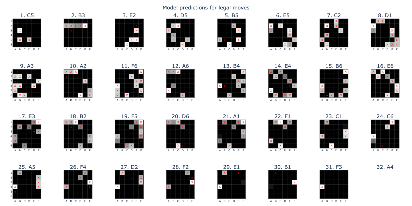
- The inputs and outputs of the model are purely textual, e.g. C5 B3 E2 D5 B5 E5..., with each of the 32 possible moves encoded as a unique token.
- The model outputs a distribution across all 32 moves and we measure accuracy on the top-1 logit.

Fig 1a. A sample 6x6 Othello game with legal moves at each game position marked 'x'.

Fig 1b. OthelloGPT predictions for possible next moves.

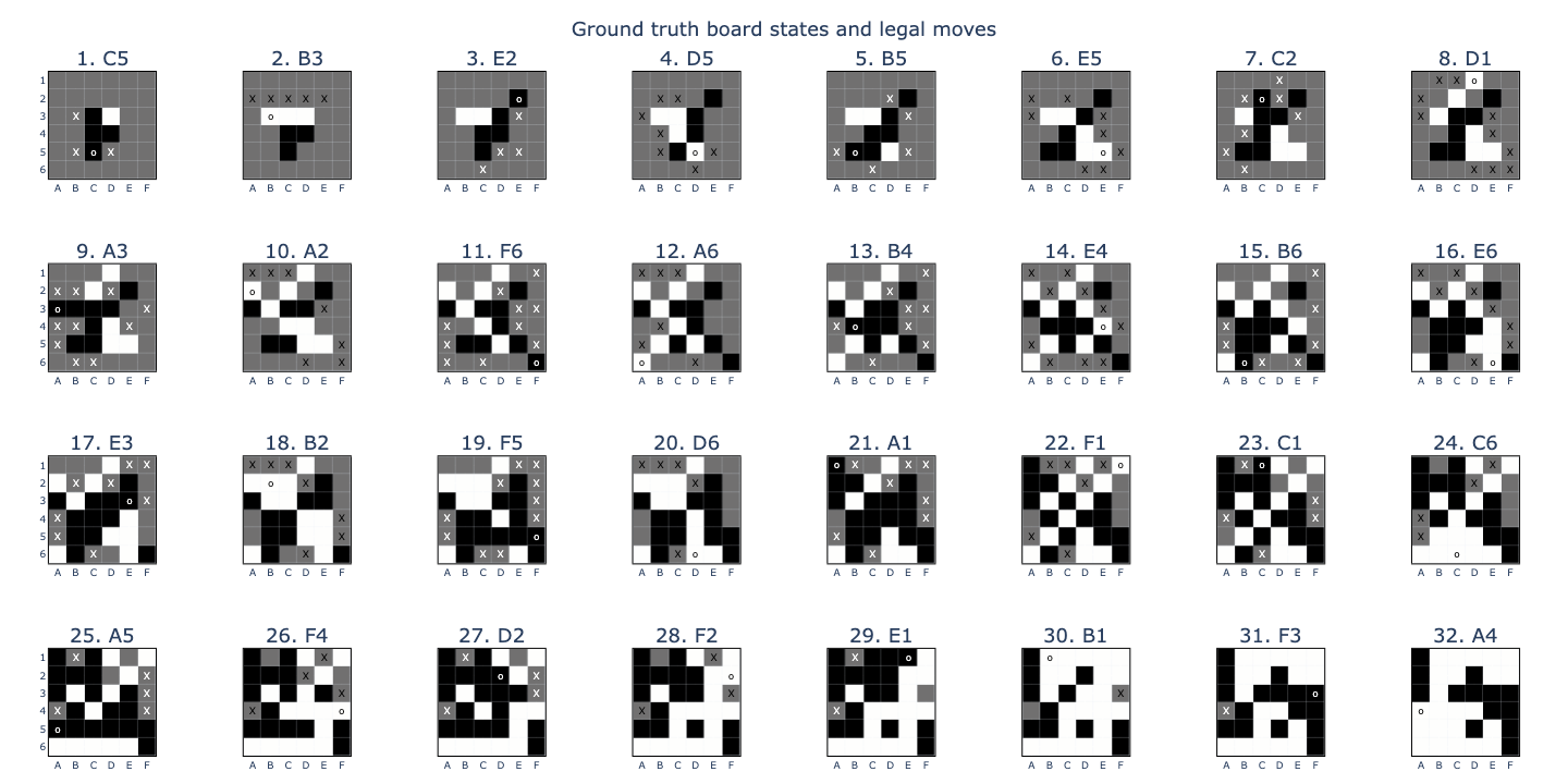
A setup for training linear probes: matrices that map from OthelloGPT’s residual stream to board state targets.
- The residual stream consists of vectors \(\mathbf{x}_p^{(l)} \in \mathbb{R}^{256}\) at each move position \(p \in \{0, \ldots, P-1\}\) and layer \(l \in \{0, \ldots, L-1\}\) that are produced by OthelloGPT at inference time.
- At each position, we have information \(\mathbf{y}_p \in \{0, \ldots, K-1\}^{36}\) on the state of each square on the board, e.g. whether a square is \(white\) (0), \(empty\) (1), or \(black\) (2). We call these targets.
- In a given game, we have a target matrix \(Y \in \{0, \ldots, K-1\}^{36 \times P}\) and inputs \(X^{(l)} \in \mathbb{R}^{256 \times P}\) for layer \(l\). We use logistic regression to train a linear map \(M^{(l)}: X^{(l)} \mapsto \hat{Y}\) from residual stream vectors to logits \(\hat{Y} \in \mathbb{R}^{36 \times P \times K}\). We call this a linear probe for layer \(l\) and we train a separate probe for each layer in the model, including “middle” layers in between the attention block and MLP, referred to as L0_mid or L0.5, etc.
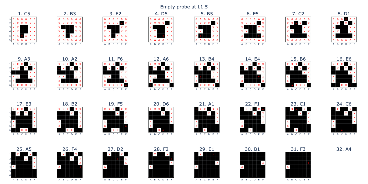
A binary linear probe (EE) that predicts whether a board square is \(empty\) with 99.99% accuracy at L1_mid.

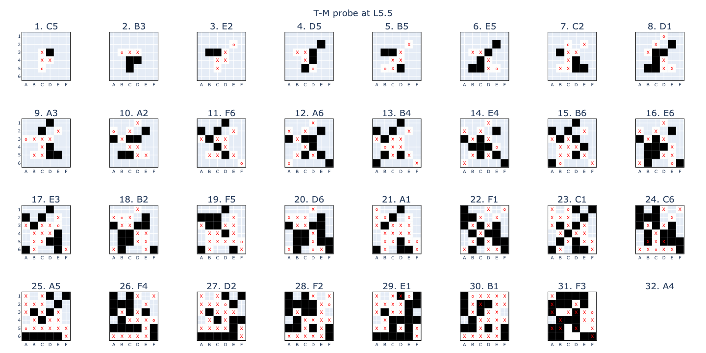
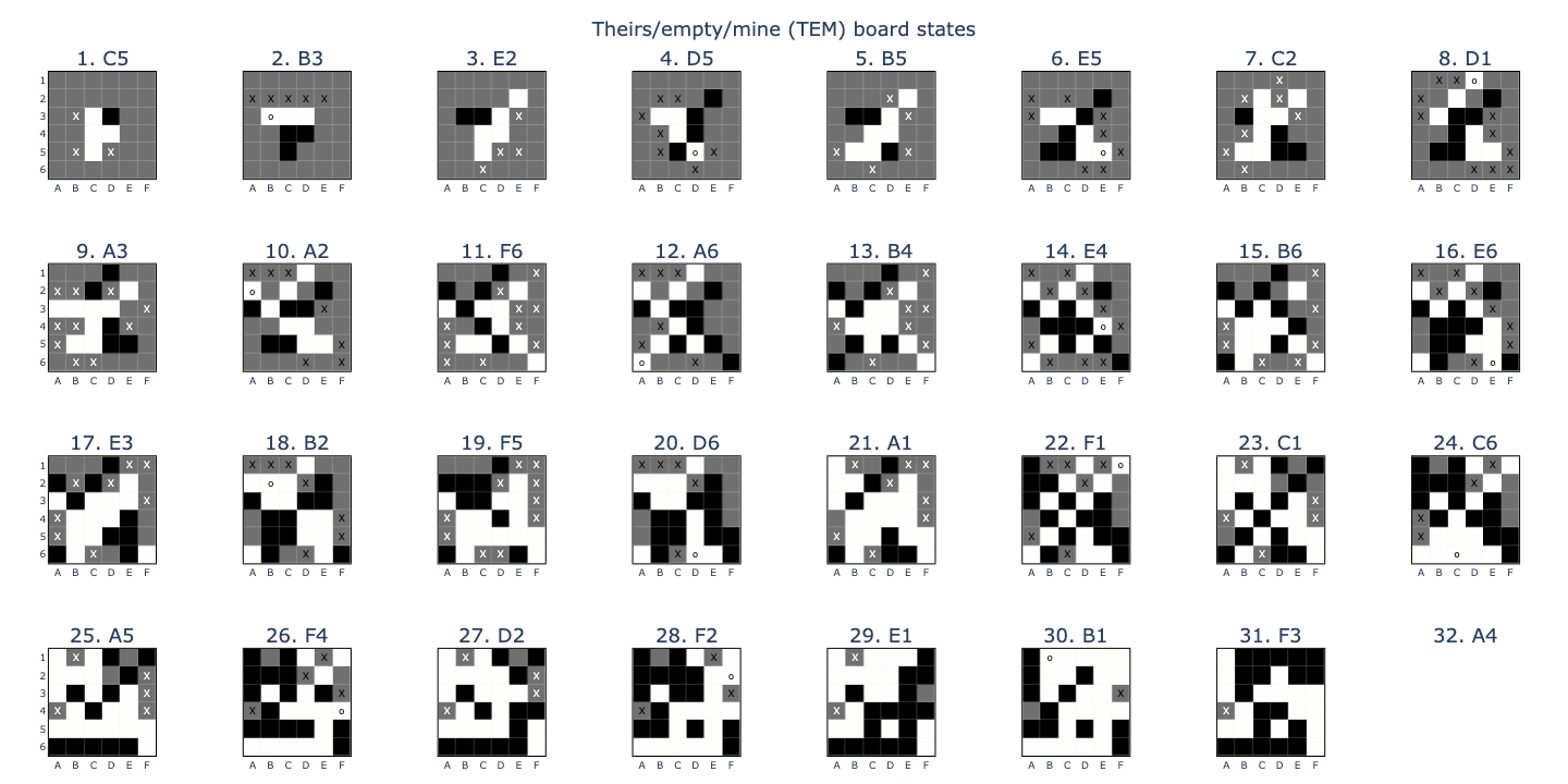
Fig 2. (EE) probe predictions for empty board squares at each position.

A binary linear probe (T-M) that predicts whether a non-empty board square belongs to the opponent, i.e. is \(theirs\) (T) and not \(mine\) (M), with 99.1% accuracy at L5_mid.

Fig 3. (T-M) probe predictions for whether a non-empty board square is theirs/mine.

A setup for visualising vectors under the basis transformation defined by a binary linear probe.
- For a binary probe \(M: \mathbb{R}^{256} \rightarrow \mathbb{R}^{36 \times 2}\), I interpret the vector M[:, i, 1] as the direction in the residual stream space that aligns with the target feature for square \(i\), where \(i=0\) for A1, \(i=1\) for A2, etc.
- This allows us to transform any vector \(\mathbf{x} \in \mathbb{R}^{256}\) into a 6x6 image corresponding to a board state representation. For example, I previously transformed the input weights \(\mathbf{w}_i\) and output weights \(\mathbf{w}_o\) for a specific neuron, showing that it activates strongly on a board state where F2 is \(empty\), F3 is \(theirs\), and F4 is \(mine\), and then outputs that F2 is a legal move!

Fig 4. Neuron L5N415 weights visualised in various probe bases.

A question and a hunch

I wanted to build on this work, but this was also my first attempt at doing mech interp research. Rather than answering high level questions, such as “what makes a good feature?” or “how do we interpret superposition in transformers?”, I went with a more practical approach. I set out to answer the question: “how does OthelloGPT compute its world model?”

The circuits and features discovered so far were focused on the tail end of the model’s computation: extract the linearly represented board state and show how it’s used to compute logits. I had a hunch that the model was using additional latent features in order to compute the board state in the first place. There was some weak evidence for this:

At the end of my previous post, I noticed colinearities between the board state probes (EE & T-M) and the unembedding vectors (U). I saw this by visualising W_U in the (EE) and (T-M) bases, showing for example that (U)_A1 was highly colinear with (EE)_A1, (T-M)_B2, and ~(T-M)_C3: board states that are highly correlated with but not equivalent to A1 being a legal move.

Fig 5. (W_U) visualised in the (EE) and (T-M) probe bases.

The repertoire of feature vectors so far amounted to at most 163 dimensions out of 256 available.

Feature vector	Count
Token embed (B)	32
Pos embed (P)	31
Empty probe (EE)	32
Theirs/mine probe (T-M)	36
Token unembed (U)	32
Total	163

If this were the entire feature set, it would be possible for the model to represent these features as linearly separable monosemantic directions. The question is whether the model is sufficiently incentivised to do this. We’ve seen neurons which output legal logits using these board state features, so it seems that the superposition with (T-M) in particular could lead to some undesirable confounding.

An alternative explanation is that the model does all its legality computations in parallel, after which it no longer needs to maintain an accurate board state representation. Thus it’s never necessary to represent the features simultaneously.

Either way, I decided that it would be useful to pursue the hunch and see if it was possible to find some interesting probes. I came up with two theories that could lead to additional features.

Inductive theory

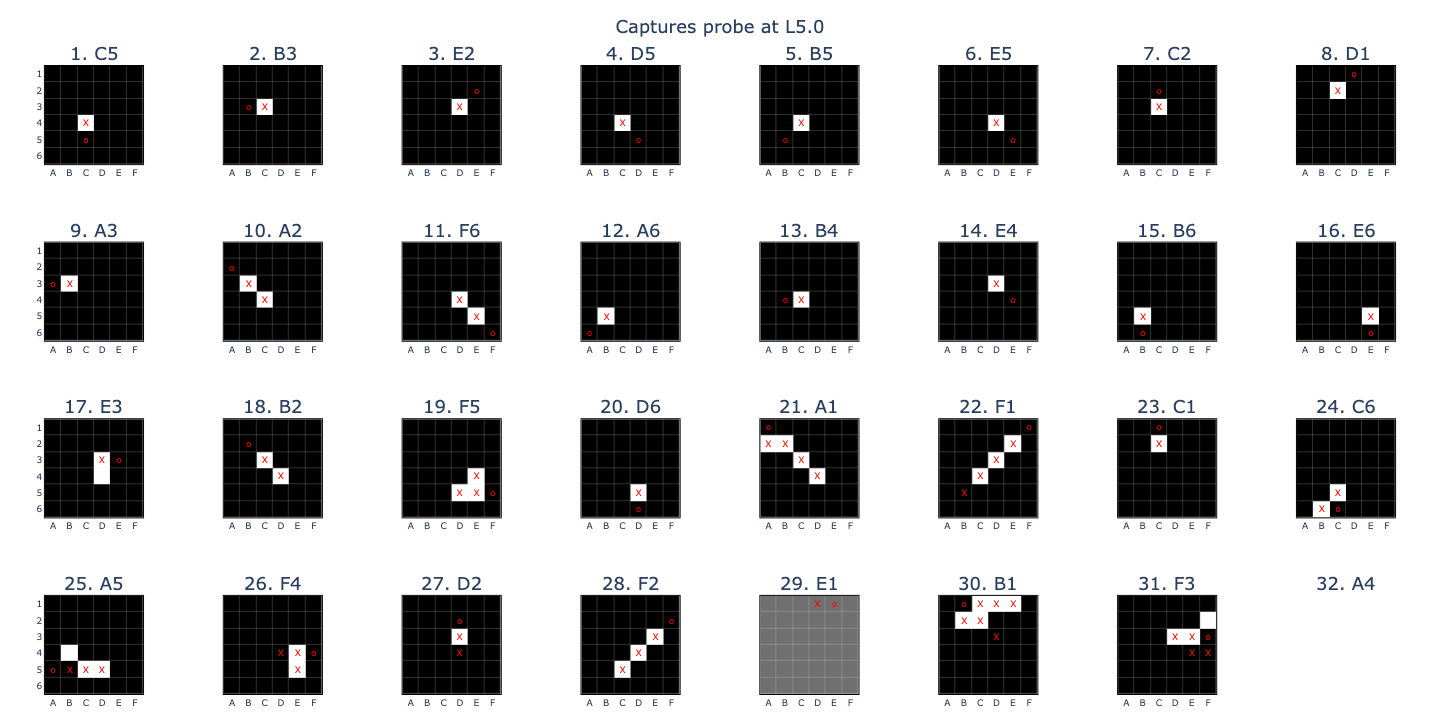
My first idea was that OthelloGPT could be working out board states inductively: layer by layer, it could take the current board, apply the next move, flip a bunch of tiles, and continue. In order to do so, it would use board state features corresponding to the \(previous\) board state (PTEM), as well as another feature corresponding to \(captured\) (C) squares.

Fig 6a. A sample game with board states represented as theirs (black), empty (grey), or mine (white).

Fig 6b. (PTEM) probe predictions targetting whether a square was previously theirs/empty/mine. Note that the colours are flipped vs Fig 6a; what's 'mine' now was 'theirs' in the previous player's view.

Fig 6c. (C) probe predictions targetting which squares were captured by the previous move.

The inductive logic for calculating a square’s current state from the previous one would then be:

(PT) -> (T): the opponent’s squares cannot be captured by their own move
(PM) + (C) -> (T): my captured squares get flipped
(PM) + ~(C) -> (M): my uncaptured squares stay mine
(PE) -> (E) or (T): one previously empty square gets the opponent’s move played on it

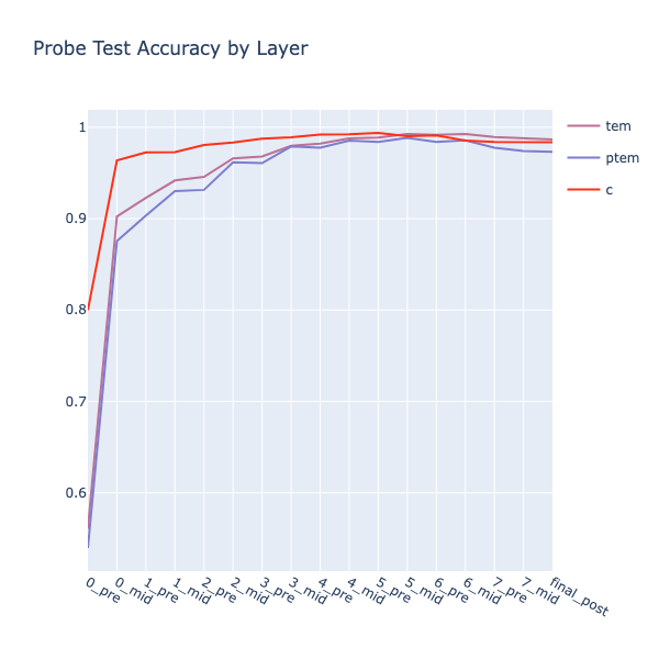
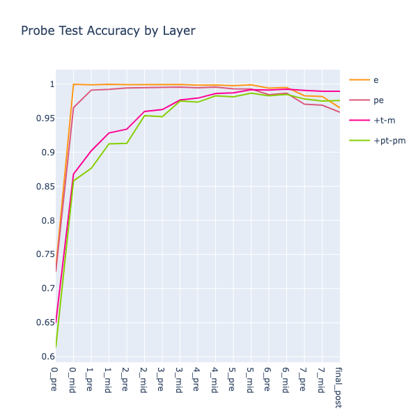
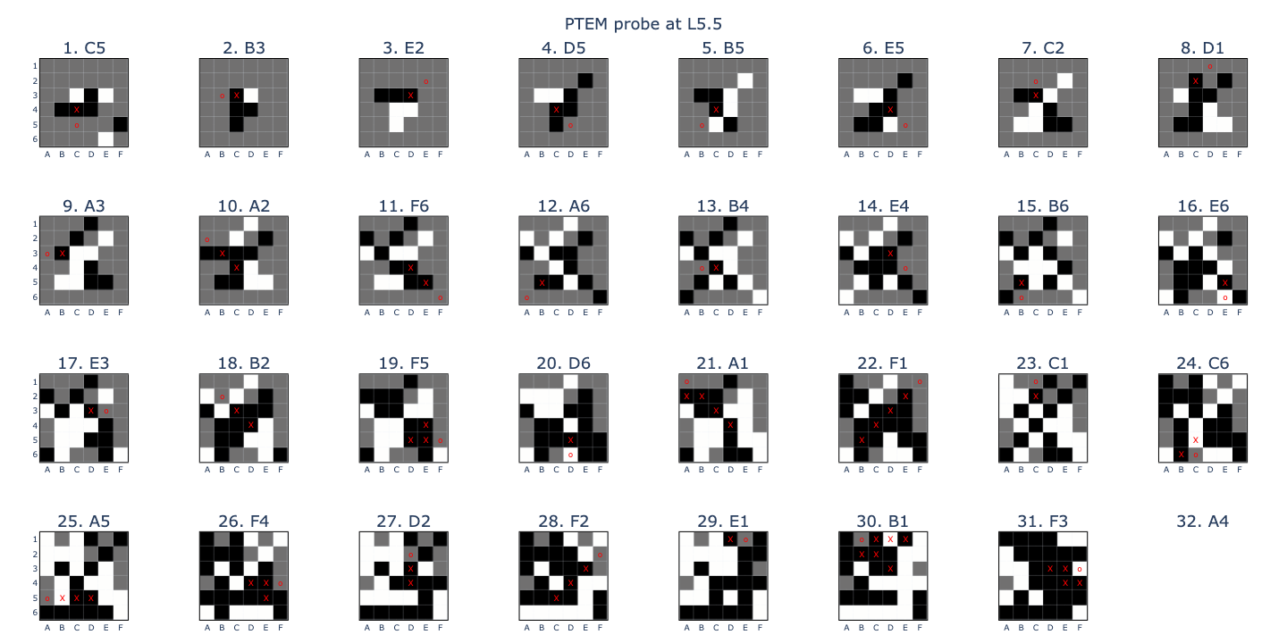
Fig 7. Probe accuracies across all layers, where the probe for each layer was trained specifically for that layer.

Ignoring pos 0 in the accuracy calculations (I hoped that if I didn’t prepend the initial board state to the training data, the probes would find the model’s representation of it at pos 0, but this didn’t work), the (PTEM) probes performed almost as well as the original (TEM) probes!

Conditional theory

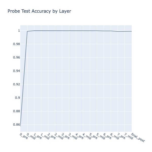
These inductive probes were cool, but this logic would require 31 layers to compute all board positions. Yet, judging from the accuracy plots, OthelloGPT seemed to suffice with just 5. This meant that it had to be calculating board state elements across multiple positions in parallel. One clear example was the \(empty\) (E) state, which was computed across all game positions and board squares after just one attention layer!

I figured that the model had to be separating out the simplest possible features for each square, computing each one in parallel, at the earliest layer possible, and then combining them in later layers. For example, the \(captured\) (C) feature could be initialised as a maximum likelihood prior across all squares that a move could potentially capture and then refined over subsequent layers (it’s not possible to capture (E) squares, etc.). This greedy approach could explain the better-than-random probe accuracies at L0, immediately after embedding.

The combination of these simple probes into useful outputs would then be done via conditional statements. For example, only \(empty\) (E) squares can be \(legal\) (L), and only ~(E) squares can be \(theirs\) or \(mine\) (T-M).

Fig 8. A decision flowchart for combining simple features using conditional logic in OthelloGPT.

These combinations could be expressed as linear functions across token positions using attention heads, or as non-linear functions within the same position using neurons. For example, we previously saw that once the board state was computed at each position, neurons could be used to find legal moves. But in other cases, such as predicting the final move in a game, an attention head might be more suitable for finding all previous moves and outputting the remaining empty square as the only possible move.

This idea led me down a rabbit-hole of training a lot of probes which were ultimately not very useful, but I think the underlying intuition is still nice! It suggests an intelligence paradigm more akin to how a highly parallelised, probabilistic machine brain would think, as opposed to a human one.

Sprint

At this point, I was getting pretty bogged down in the project. I felt I hadn’t really discovered anything concrete, the messy code was piling up, and my latest investigations had been frustratingly unfruitful. I decided to use the application process to Neel’s MATS stream as a forcing function to get something done in a 16-hour sprint.

This made me choose an even narrower project scope. Instead of figuring out how the entire board state was computed, I decided to focus in on just the \(empty\) (E) state.

Revisiting the PE probe

While investigating my Inductive Theory, I trained a \(captured\) (C) probe with the relationship (T-M) = (PT-PM) + (C). I hypothesised that a similar relationship could be found linking (E) and (PE) - the difference between the two is exactly one previously empty square on which the latest move was played. I trained binary probes (EE) and (PEE) that targeted only whether squares are empty or non-empty, ignoring other information.

def empty_target(batch, device):
    boards = t.tensor(batch["boards"], device=device)[:, :-1]
    return (boards == 0).flatten(2)

def prev_empty_target(batch, device, n_shift=1):
    e = empty_target(batch, device)
    n_batch = e.shape[0]
    n_out = e.shape[-1]
    e0 = t.full((n_batch, n_shift, n_out), t.nan, device=device)
    return t.cat([e0, e[:, :-n_shift]], dim=1)

Fig 9a. (EE) probe predictions for empty board squares at each position.

Fig 9b. (PEE) probe predictions for empty board squares at the previous position.

Fig 9c. Probe accuracies for all probes targetting empty board states. The (PE) and (PEE) lines overlap.

Since both probes had very high accuracies, I just worked with the normed difference vector (PEE-EE) instead of training a new prob explicitly targetting the latest move. Using this (PEE-EE) basis as a transformation for the embedding weights (W_E) showed that the probe could indeed extract the move that each token embedding was representing!

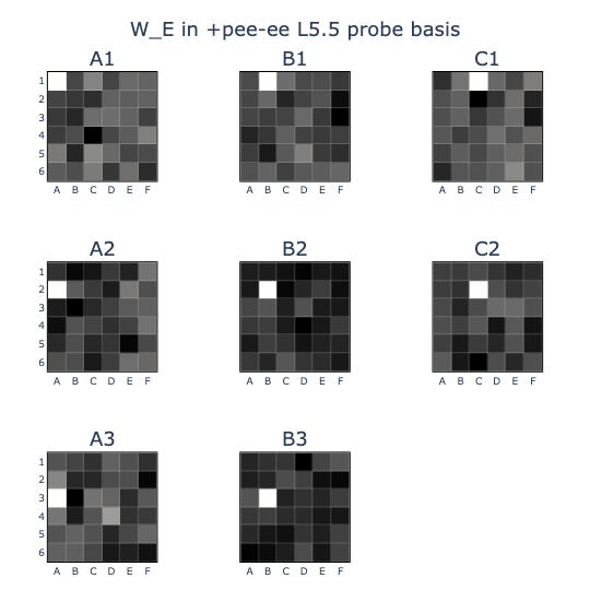
Fig 10. (W_E) visualised in the (PEE-EE) probe basis.

This was sufficient information for computing the (EE) board state using just one layer: all the model had to do was see which moves hadn’t yet been played at each position and mark these as (EE). And all I had to do was find the attention heads that did this…

Finding L2H5

I used two tools here to identify attention heads that were writing out (EE) vectors. The first was Neel’s TransformerLens library, which I used to cache the decomposed residual stream vectors being written by each attention head across 200 forward passes of the model.

input_ids = t.tensor(test_dataset["input_ids"][:200], device=device)
_, cache = model.run_with_cache(input_ids[:, :-1])
X, y_labels = cache.get_full_resid_decomposition(
    apply_ln=True, return_labels=True, expand_neurons=False
)
X /= X.norm(dim=-1, keepdim=True)

The second tool was an SVD calculation to find the amount of variance that was explained by a given probe basis. I ran into numerical instability issues when passing highly colinear probes into the function, so I added some checks for this.

def calculate_explained_var(
    X: Float[t.Tensor, "batch ... d_model"],
    b: Float[t.Tensor, "d_model basis"],
):
    # Use double precision (not supported by mps) to minimise instability errors
    # Alternatively add a jitter term
    X = X.detach().cpu().double()
    b = b.detach().cpu().double()

    # Add a small regularisation term to b to perturb it
    b += 1e-6 * t.randn_like(b)

    # Perform SVD on the basis vectors to get an orthonormal basis
    U, S, _ = t.linalg.svd(b, full_matrices=False)

    # Calculate the conditioning number
    condition_number = S.max() / S.min()
    cond_threshold = 1e6
    if condition_number > cond_threshold:
        print(f"Condition number: {condition_number}")
        print(S / S.min())
        U = U[:, (S / S.min() > cond_threshold)]

    # Project X onto the orthonormal basis
    proj = t.matmul(X, U)

    # Reconstruct the projections
    proj_reconstructed = t.matmul(proj, U.transpose(-1, -2))

    # Compute the squared norms of the projections and the original vectors
    proj_sqnorm = t.sum(proj_reconstructed**2, dim=-1)
    X_sqnorm = t.sum(X**2, dim=-1)

    # Calculate the explained variance ratio
    explained_variance = proj_sqnorm / X_sqnorm

    # Take the average over the batch
    explained_variance = t.mean(explained_variance, dim=0)

    return explained_variance

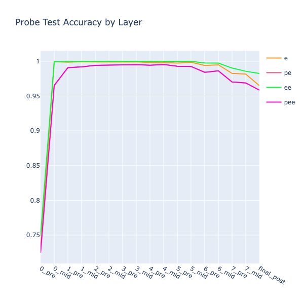
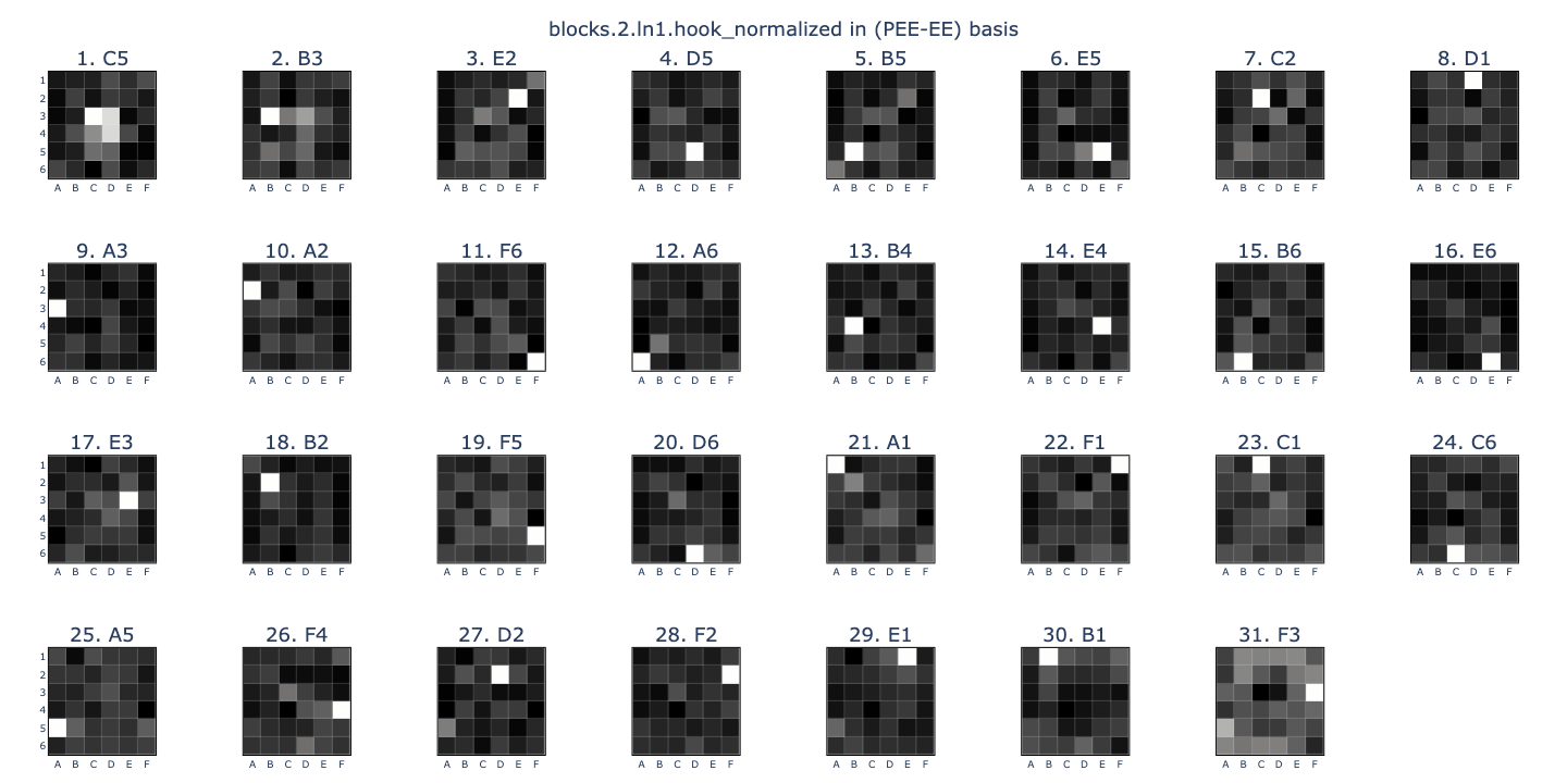
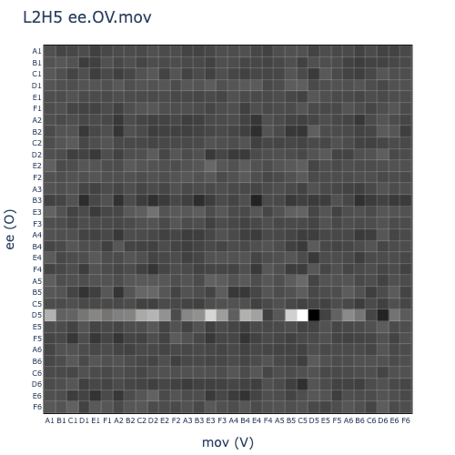
I used these tools to visualise how much of the decomposed residual stream at each position was explained by the 32-dimensional (EE) basis, averaged across the batch.

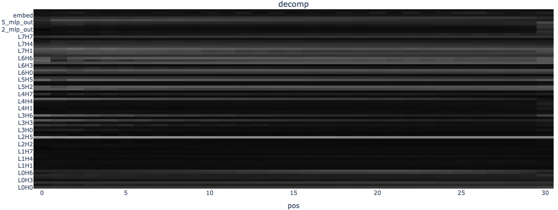
Fig 11. A heatmap showing the percentage of output variance from each OthelloGPT component that is captured by the (EE) basis, averaged across a batch of 200 games.

As expected, the L0 heads were fairly active in this basis, as were the L7 heads. I interpreted the latter as a computation in (U) space that spilled over into (EE) space due to colinearities, but investigating this was out of scope. Interestingly, L2H5 was the highest in explained variance, so I looked at some sample attention patterns using circuitsvis.

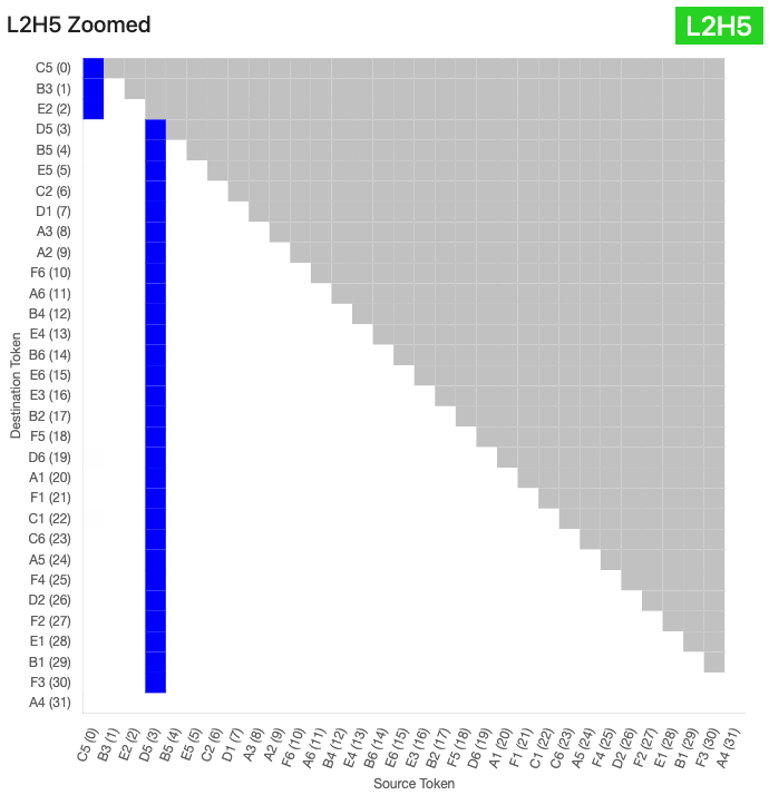
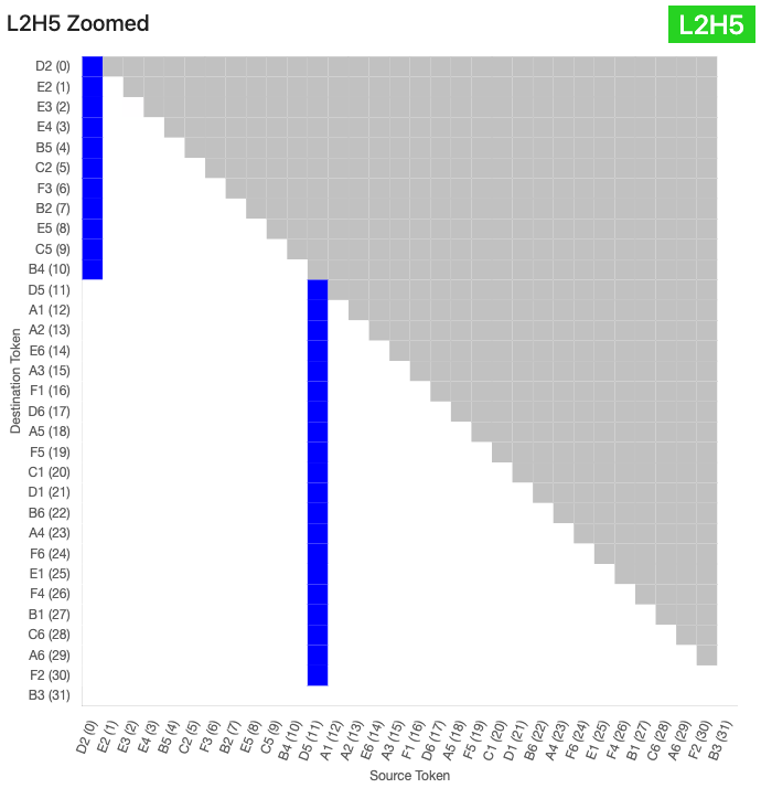
Fig 12. Attention patterns for L2H5 sampled from 2 random games.

It looked like L2H5 attended specifically to the D5 token, otherwise defaulting to pos 0. I re-ran the explained variance calculation with just the probe for the D5 square, instead of all 32 (EE) probes, and saw that this single vector accounted for over half of the output variance!

Fig 13. A heatmap showing the percentage of output variacne from each OthelloGPT component that is captured by the singular (EE)_D5 vector, averaged across a batch of 200 games.

Interpreting L2H5

Although I couldn’t explain why a whole L2 attention head was seemingly being used to recompute the (EE) state for D5 (assuming that it had already been calculated after L0), I decided to go ahead with interpreting it anyway and deal with that question later.

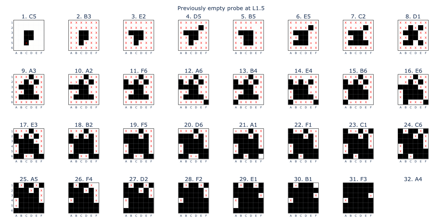
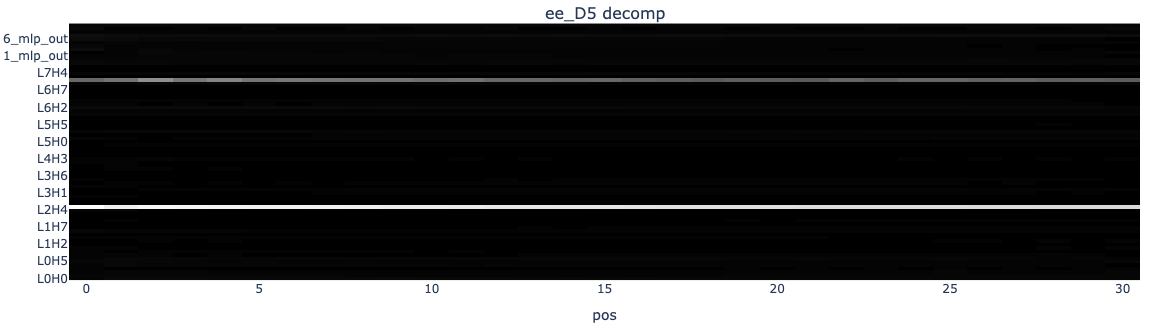
Firstly, I checked whether the (PEE-EE) probe was still able to extract the latest move from each position at L2_pre by taking a cached game and transforming the residual vector at each position using the probe.

Fig 14. A sample residual stream input to L2H5 visualised in the (PEE-EE) basis at each position.

Success! Recall that we previously interpreted neurons by transforming their input and output weights into probe bases. Interpreting attention heads required a slightly different approach. Following Anthropic’s mathematical framework, attention heads can be separated into two bilinear forms (W_QK) and (W_OV), where

\[A = softmax(\mathbf{x_{dst}} W_Q^T W_K \mathbf{x_{src}})\] \[\mathbf{x_{out}} = (A \otimes W_O W_V) \cdot \mathbf{x_{src}}\]

Thus, it should be possible to probe each individal weight matrix to see how they align with certain features across head dimensions. If a head wants to attend to source tokens with a given feature, (W_K) should align with that feature vector. If it wants to output another feature, its vector should be seen in (W_O), etc. I found interpreting these results more difficult than with the neurons because there were multiple head dimensions, compared to the single scalar activation value for each neuron, so it was possible that linear combinations were being taken across head dimensions.

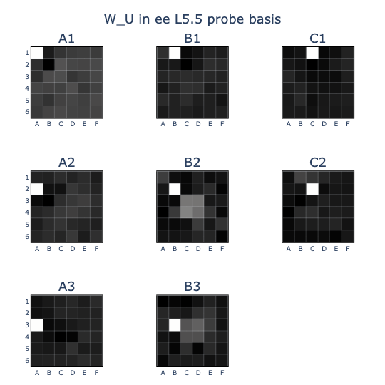
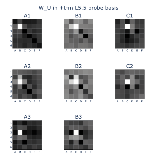
I probed L2H5’s (W_K) with (PEE-EE) and the \(positional\) (P) embedding, expecting to see strong alignment with (PEE-EE)_D5 and (P)_0. Note: the (P) images are arranged into board squares by my visualisation function but in this case it doesn’t mean anything.

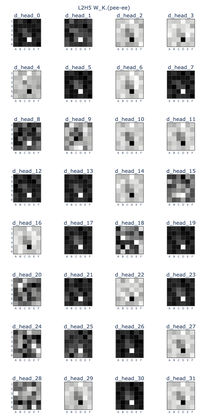
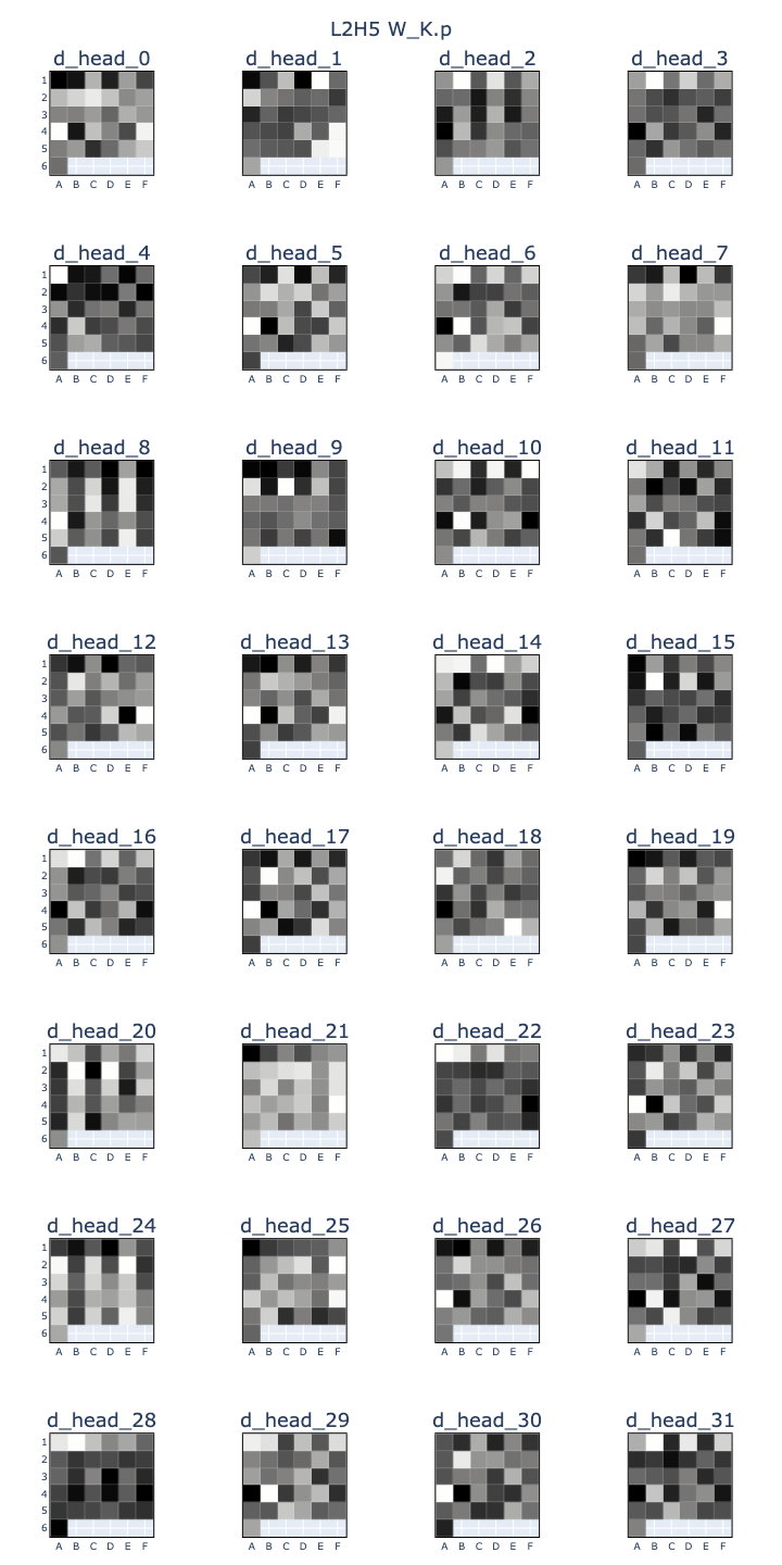
Fig 15. L2H5 (W_K) visualised in the (PEE-EE) and (P) bases, across all 32 head dimensions.

These images were difficult to interpret. While (W_K) was well aligned with (PEE-EE)_D5, many of these alignments were negative, and the images generated by the (P) transform were even less informative.

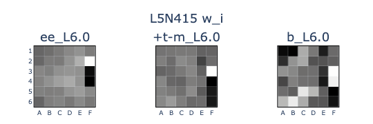
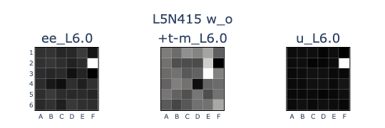
Next, I probed L2H5’s (W_V) with (PEE-EE) and (P), and also probed L2H5’s (W_O) with (EE), expecting to see activations in (W_V) for (PEE-EE)_D5 and (P)_0 and activations in (W_O) for (EE)_D5.

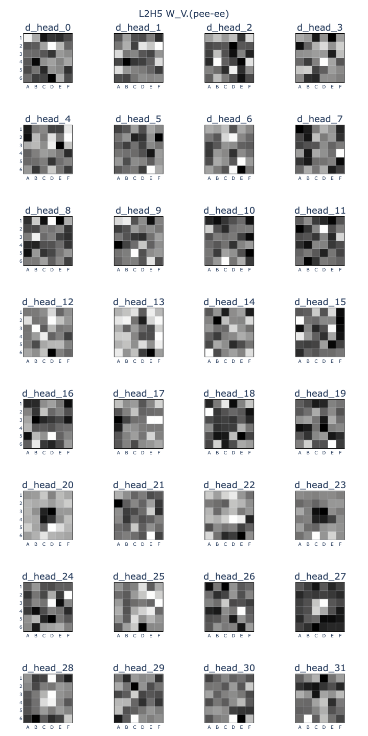
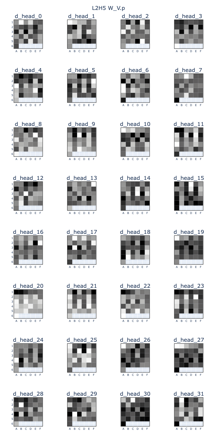
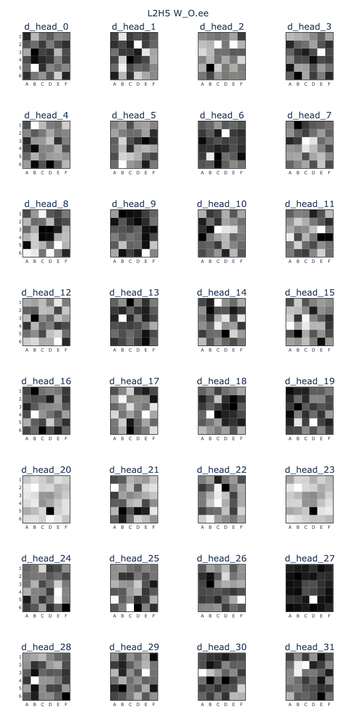
Fig 16a. L2H5 (W_V) visualised in the (PEE-EE) and (P) bases, across all 32 head dimensions.

From the (W_O) transformations, I could roughly see that dimensions 19 & 27 wrote out (EE)_D5 and dimensions 20 & 23 wrote out ~(EE)_D5. Matching these up to the (W_V) images was difficult - a better visualisation was required.

Improvements

The sprint was completed under pretty tight time constraints, so a lot of the decisions I made were suboptimal and the original conclusion was fairly lacklustre. After it ended, I made a few quick clean-ups that significantly improve the quality of the results.

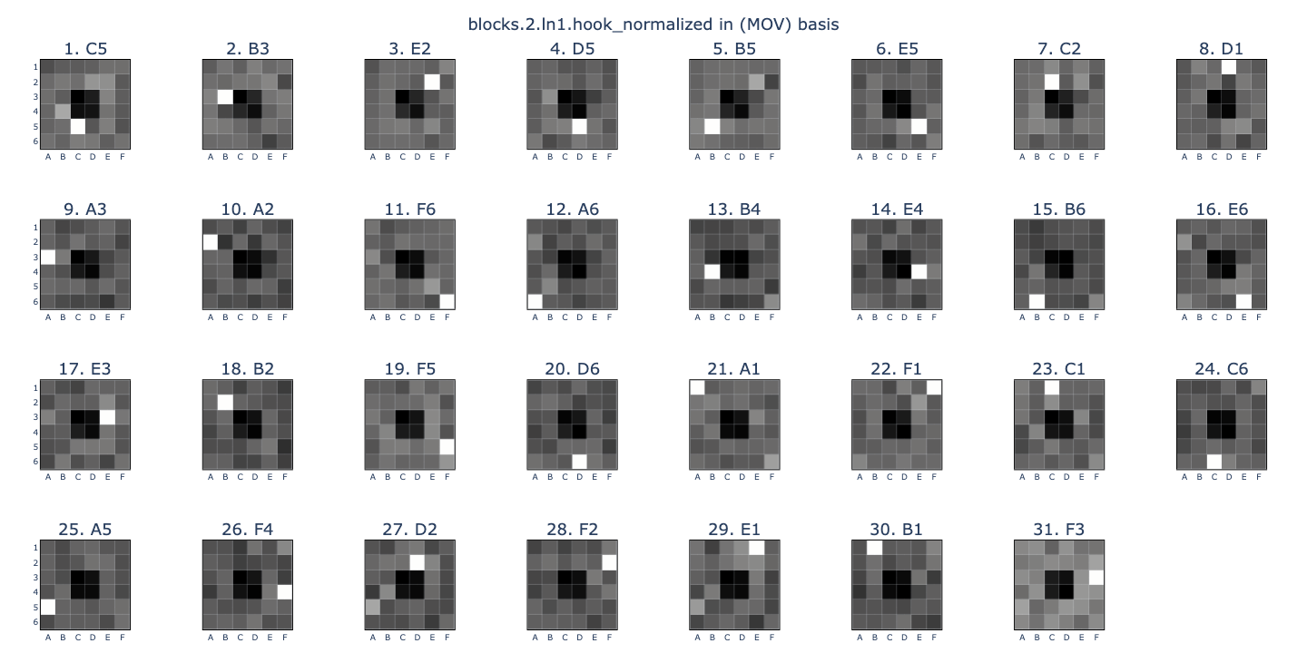
MOV probe

Firstly, I replaced the (PEE-EE) probe with a new probe trained directly to target the \(latest\ move\) (MOV). The probe was accurate across all layers.

Fig 17a. A sample residual stream input to L2H5 visualised in the (MOV) basis at each position.

Fig 17b. (MOV) probe accuracy across all layers.

P basis

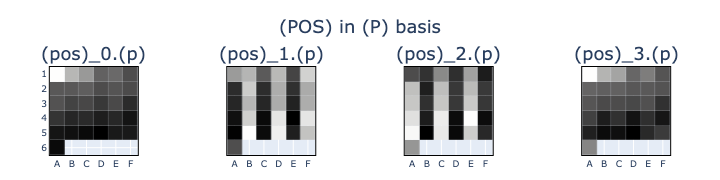
Next, checking the (MOV) probe accuracy made me realise that I had never done the same for the positional embedding (P), instead working on the assumption that it maintained its meaning across all layers. In fact, (P) only has to have any meaning at L0_pre, and it’s possible that it loses all usefulness once the model encodes moves into the \(theirs/mine\) basis. I visualised a sample residual stream at L0_pre, L0_mid, and L2_pre through a (P) transformation and saw that this seemed to be the case.

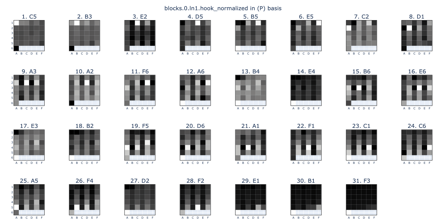
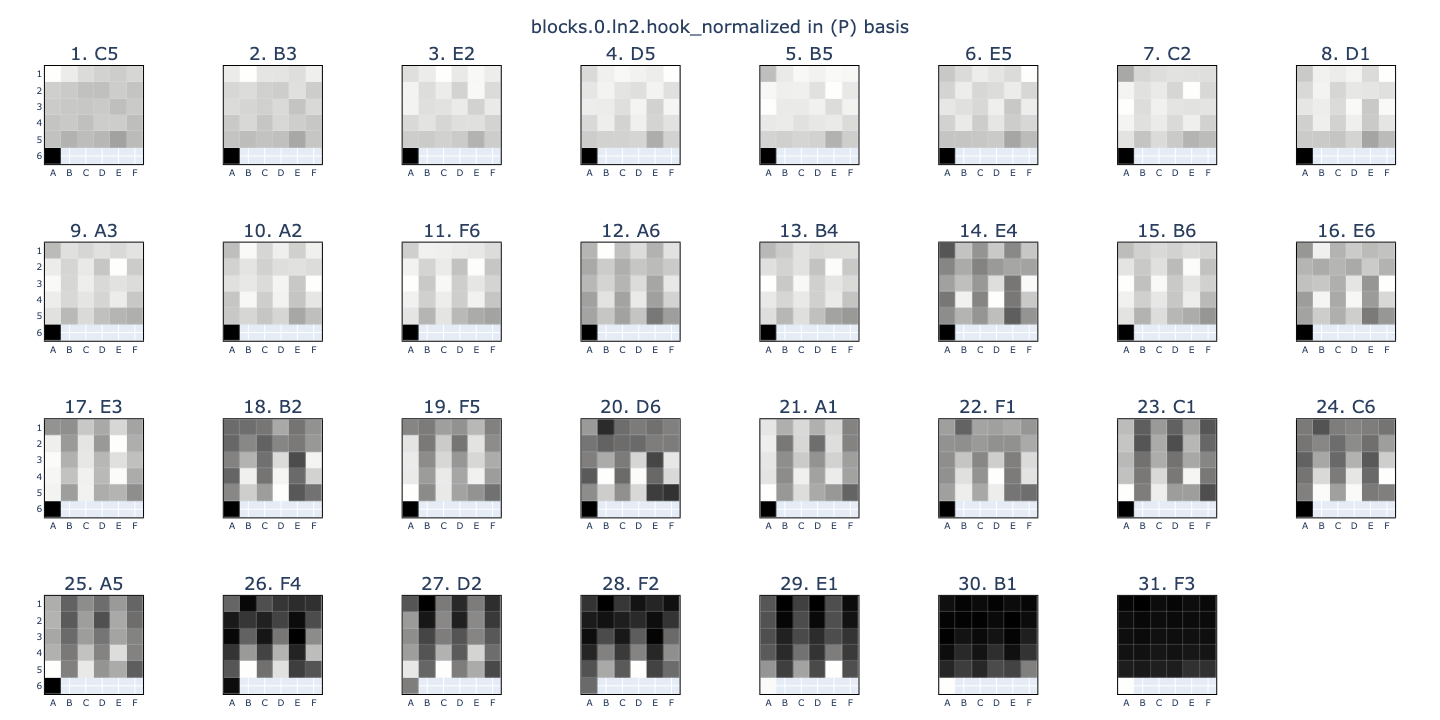
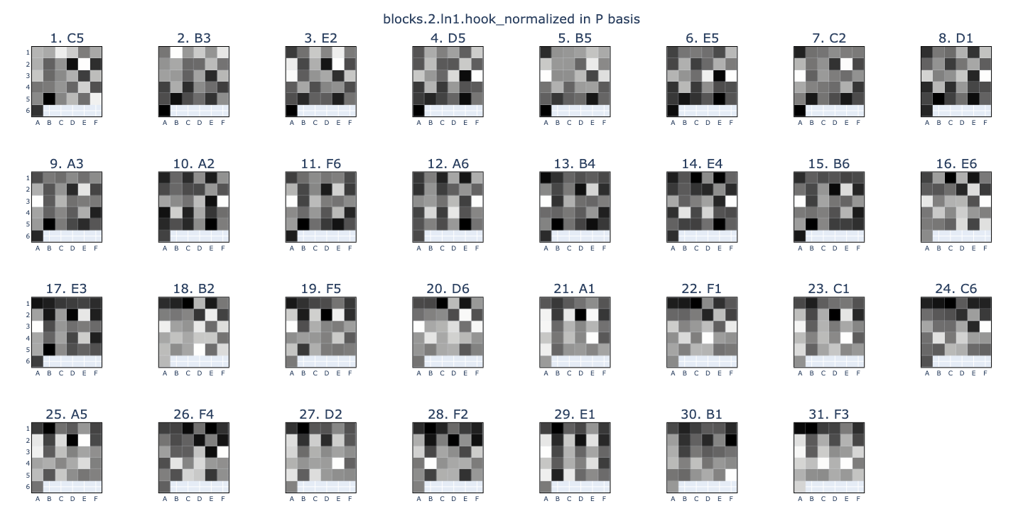
Fig 18b. A sample residual stream at L0_mid visualised in the (P) basis at each position.

Fig 18c. A sample residual stream at L2_pre visualised in the (P) basis at each position.

By the time we get to the input for L2H5, (P)_0 has no discernible meaning at all! I was sure that the model still needed some positional information, so I trained a new positional probe (POS) with 4 binary targets: pos 0 (0), pos odd (1), pos even (2), pos last (3).

def pos_target(batch, device):
    input_ids = t.tensor(batch["input_ids"], device=device)[:, :-1]
    y = t.zeros((*input_ids.shape, 4), device=device, dtype=int)
    y[:, 0, 0] = 1      # pos 0
    y[:, 1::2, 1] = 1   # pos odd
    y[:, ::2, 2] = 1    # pos even
    y[:, -1, 3] = 1     # pos last
    return y

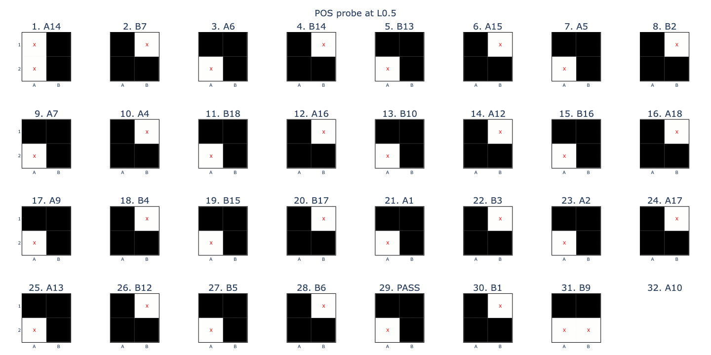
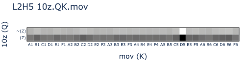
Fig 19a. (POS) probe predictions at L0.5 (ignore the subplot titles).

Fig 19b. (POS) probes visualised in the (P) basis.

(POS) was 100% accurate between L0.5 and L6! This gave me a consistent, meaningful vector (POS)_0 targetting tokens at pos \(0\), which I named (Z). With these improved probes, I went back to L2H5 and applied them to (W_K) and (W_Q).

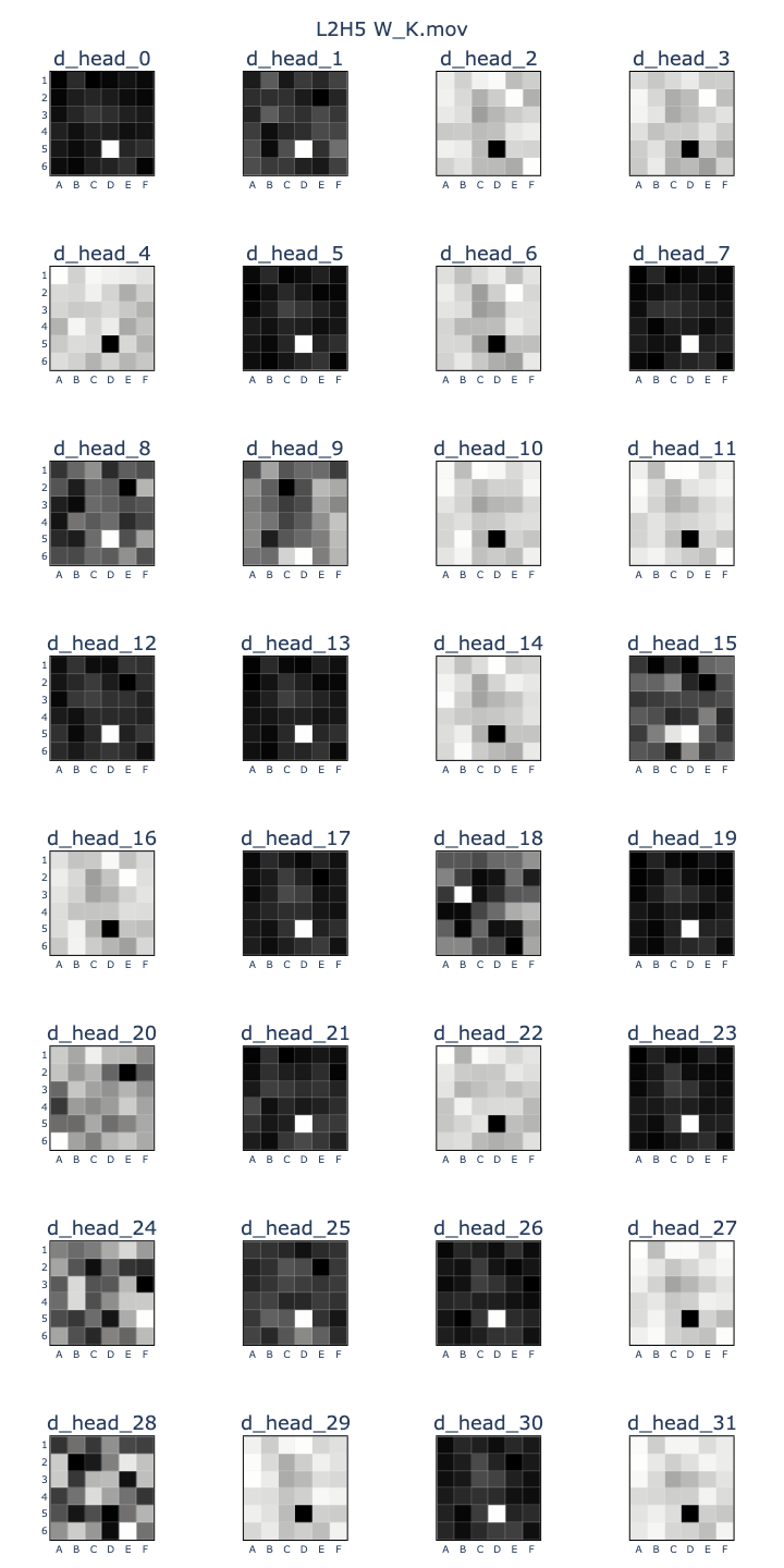
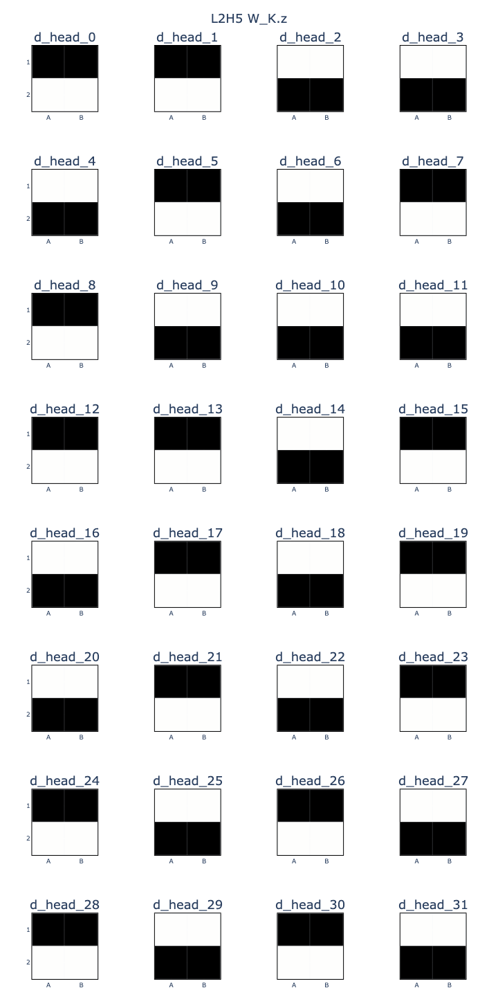
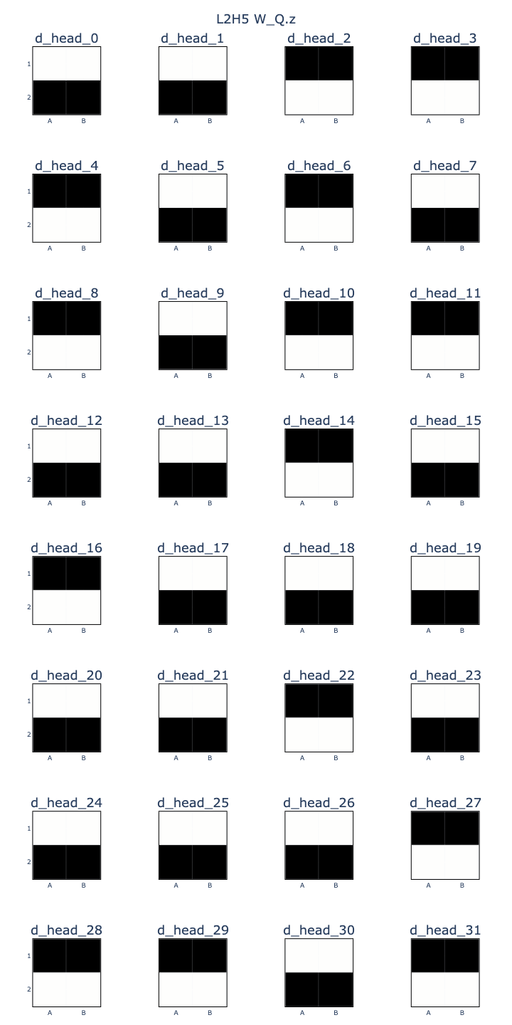
Fig 20. (W_K).(MOV), (W_K).(Z), and (W_Q).(Z), with (Z) re-arranged such that row 0 = ~(Z), row 1 = (Z).

Success! We can now see a pattern that suggests that the QK circuit broadly attends to (MOV)_D5 keys from ~(Z) queries, and vice versa. Additionally, the head dimensions in (W_K) that align positively with (MOV)_D5 also align positively with (Z), providing a mechanism for attending to keys with (MOV)_D5 or (Z), subject to scaling and causal masking.

Bilinear visualisation

Finally, I revisited the attention head weights visualisation. Instead of probing each (W_K), (W_Q), etc. independently, I applied the probes to each side of the full bilinear forms and plotted the resulting matrices. This helped to remove some ambiguity about how the head dimensions would interact with each other in the dot product.

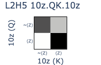
Great success! After scaling the normed (Z) vector by 10x (which I think is necessary because this OthelloGPT model was trained with bias terms), we finally get the expected images that depict linearly separable mechanisms in L2H5.

QK circuit:
- Queries originating from ~(Z) tokens attend strongly to (MOV)_D5 keys: tokens where the move D5 was played.
- In the absence of a (MOV)_D5 key due to causal masking, there is a preference for (Z) keys: tokens corresponding to pos 0.
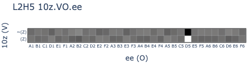
OV circuit:
- A (Z) value token, and many ~(MOV)_D5 values, will output (EE)_D5.
- ~(Z) and (MOV)_D5 values will output ~(EE)_D5.

Conclusion

My goal for the project was to find evidence for additional probes and use them to interpret an attention head for computing the board state. I didn’t quite accomplish this in the sprint, but after the follow-up I’d say I managed it!

I found three new probes, corresponding to squares that were just \(captured\) (C), the latest played \(move\) (MOV), and a compressed \(positional\) (POS) basis. I extracted the pos \(0\) (Z) probe from (POS).
I used cached outputs from each attention head and an explained var calculation to see that L2H5 writes out vectors that are aligned with (EE)_D5 in most forward runs.
I showed that the L2H5 QK circuit uses the (MOV) and (Z) features to attend to D5 or pos 0, depending on whether D5 has been played in a previous move.
I showed that the L2H5 OV circuit writes out ~(EE)_D5 from ~(Z)/(MOV)_D5 values, respresenting the logic “if D5 has been previously played, then D5 is not empty”, and vice versa.

In terms of further work along this direction, I think it would be cool to interpret a head that computes captures. I would imagine this works by using (MOV) to attend to all previously played capturable squares and using (T-M) to identify which ones belong to the other player. I could also imagine a head that memorises common openings. For example, if a square far from the centre is played at a relatively early position, there are only a limited number of game trees that could have made this possible, which the head could categorise according to past moves. I suspect this type of work would be very much the latter part of the 80/20 rule, however.

It’s also still unclear to me why this head even exists at L2, when the (E) states are fully calculated after L0.5. A simple follow-up would be to examine the effects on board state accuracy and model performance when ablating the entire head.

As for implications for the wider field of mech interp, this work was different to existing work because it focused on attention heads rather than neurons and tried to find intermediate features with little direct relevance to the output logits. All operations within attention heads are linear, so linear probes were well suited to the task, but this also made separating out linear combinations of features somewhat difficult.

I think it would be interesting to do some follow-ups on unsupervised methods for linear feature identification. I was mostly guided by intuition and probe accuracy, and then became more confident in the probe validity as interpretable images were generated by transforming weight matrices and residual vectors. I generally defined “interpretability” as having sparse activations, implying monosemanticity. The intuition was mostly directed at how the model might generate intermediate features for use in later calculations. The following is a rough list of “things which might make a good feature”:

Intuitive meaning/purpose
Consistently high linear probe accuracy across layers
Sparse alignment with weight matrices
High alignment with forward-pass residual stream vectors
Applicability in causal interventions?

Performing a literature review after my sprint (the other way round definitely makes more sense), I found a paper on Sparse Dictionary Learning that seemed to systemise this into an unsupervised method for identifying features. If I work on this problem further, I’d like to see if I can use my experience from this project to build on this.

[1] A deep dive into OthelloGPT: Sprint

Table of Contents