This is the first part of a series on OthelloGPT and mechanistic interpretability. In this post, I’ll go over how I replicated prior work with a few small changes, resulting in a GPT that can predict legal moves in 6x6 Othello 99.97% of the time and linear probes that suggest that the model learnt to construct a representation of the board state from textual inputs. These probes will then be used to reverse engineer mechanisms within the 6M param GPT, providing insights into how transformer models think!

Table of Contents

Background

OthelloGPT is a GPT2-style model trained on Othello games, introduced by Kenneth Li et al. in 2023.¹ ² Random game sequences such as F5 D6 C5 F4 E3 C6... are fed in as textual input, where each of the 60 possible moves is represented by a unique token (A1 = 0, B1 = 1, …, H8 = 59), and the model is trained to predict the next move in the sequence. No prior structures are presented to the model, as it only works with these serially tokenised move IDs, yet it manages to predict legal moves with high accuracy. Here’s an online implementation of the base game with an AI for you to play against!

The paper showed that non-linear “probes” could be trained on the residual stream, an intermediate value vector within the model, to predict the board state after each move. Crucially, these probes could then be used to alter the model’s perception of the board state in the residual stream, changing its predictions accordingly. This was really cool because it suggested that the model constructed and used an internal world representation in order to make predictions, rather than merely memorising surface statistics, which has been a common sceptic take on how LLMs operate.

A follow-up by Neel Nanda³ showed that if you trained a probe to predict whether a square on the board was “mine” or “theirs”, rather than “black” or “white”, you could actually find a linear representation! This opened the door to mechanistic interpretations of the model, which he went on to demonstrate in great detail. Pretty much all of my replicated work is taken from here - my new discoveries will be presented in further posts.

Mechanistic interpretability is a really cool subset of AI Safety that is essentially neuroscience for AIs. As LLMs continue to explode in complexity, capability, and applicability, work such as this peels back the veil and provides transpicuous insights into what makes this latest generation of digital brains tick. I’ve been particularly fascinated with mech interp since discovering it, and with my previous experience in playing chess, I figured a project based on another board game would be a fun way to start exploring, so I got stuck in.

Replication

Base model

Self-attention has a time complexity of \(\mathcal{O}( n_l(n_cd_m^2 + n_c^2d_m))\), where \(n_l\) is the number of layers, \(n_c\) is the context length, and \(d_m\) is the dimension of the model’s residual stream. With an \(s\times s\) board, the length of the game \(n_c \sim s^2\), and the number of dimensions required to represent the board state \(d_m \sim s^2\), assuming that each square is represented by one of more orthogonal “feature” vectors. This means that inference is \(\mathcal{O}(n_ls^6)\)! As such, the first change I made was to shrink the board size down to \(6\times6\), which made repeated experimentation much more tractable whilst keeping the toy model non-trivial.

Othello Game

I generated a dataset of 2 million random game trees, not allowing passes, then used NanoGPT⁴ by Andrej Karpathy to train a 6M param GPT2-style model with 8 layers, 8 heads, 256 dimensions, and untied weights.

Why untied weights? Following the intuition from Anthropic’s Transformer Circuits post⁵, the \(W_U W_E\) circuit can be thought of as representing bigram statistics. In Othello, a move that was just played is never legal, so I thought it made sense to allow the model to learn separate representations.

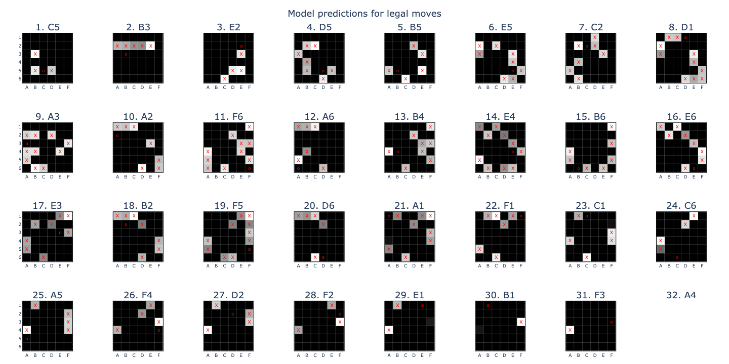
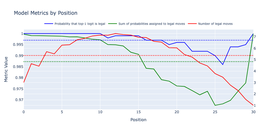
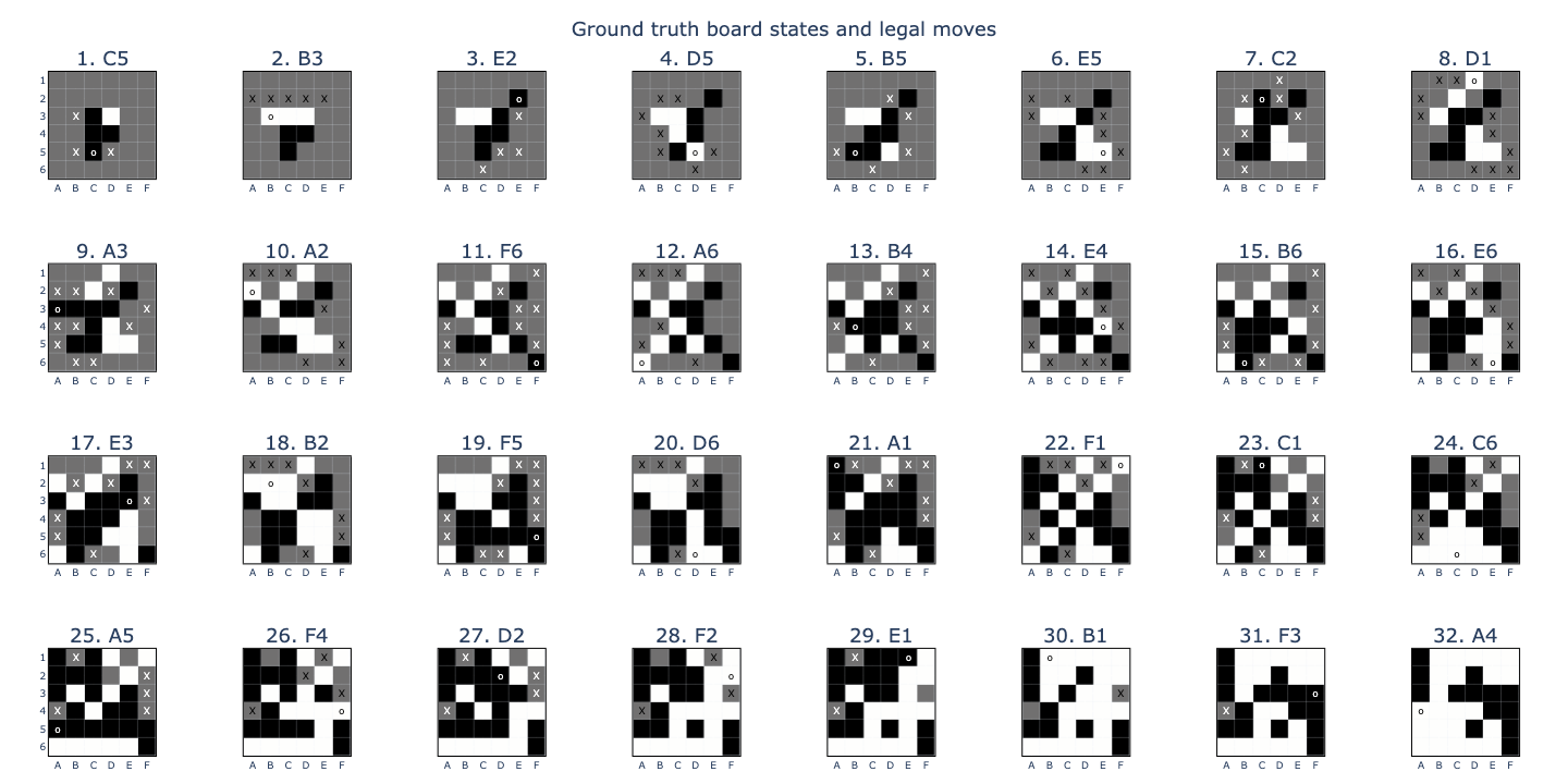
OthelloGPT Predictions OthelloGPT Metrics

Success! The model I trained had an error rate, defined as the likelihood that the top-1 logit is illegal, of 0.03%, compared with 0.01% in the original paper. Looking at the accuracies over different positions, I saw that the model’s predictions were always legal for the first 11 moves and also the final move, with its worst error rate of 1.4% on the 27th move. The likely explanation was that the model’s board state representation got less accurate as the game progressed, causing it to make more errors, until the penultimate position, where it only needed to find the last remaining non-empty square to predict the final move.

Linear probes

The probes I trained initially were linear maps \(\mathbb{R}^{d_m}\rightarrow\mathbb{R}^3\times\mathbb{R}^{s^2}\), mapping the residual stream to 3 logits per square (theirs/empty/mine). The most important thing here was setting up the training data properly - beyond this it was just a standard logistic regression.

TEM truth

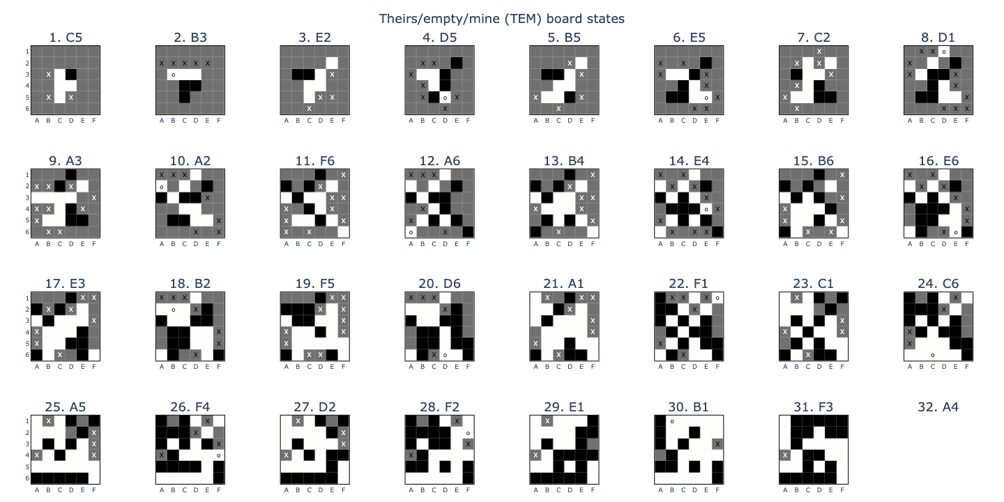
I encoded the original board states as tensors with shape \((n_c,s,s)\) and values \(+1 = black\), \(0 = empty\), \(-1 = white\). Black moves first in Othello, so after move 1, it’s white to play. In order to end up with a tensor where \(+1 = theirs\), \(0 = empty\), \(-1 = mine\), all I had to do was flip the signs for every odd position, i.e. board[1::2] *= -1. The smaller board allowed me to train probes for every layer all at once, including “middle” layers in between attention heads and MLP layers. Thus, the full probe’s weight tensor had shape \((d_m, 2n_l+1, 3, s^2)\).

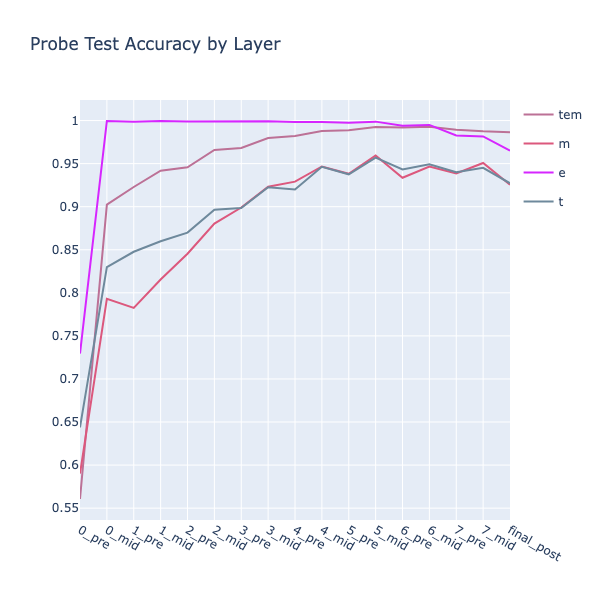
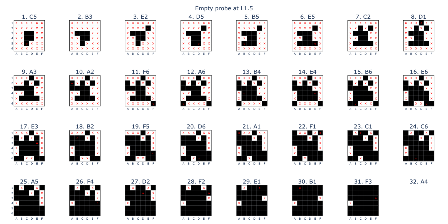
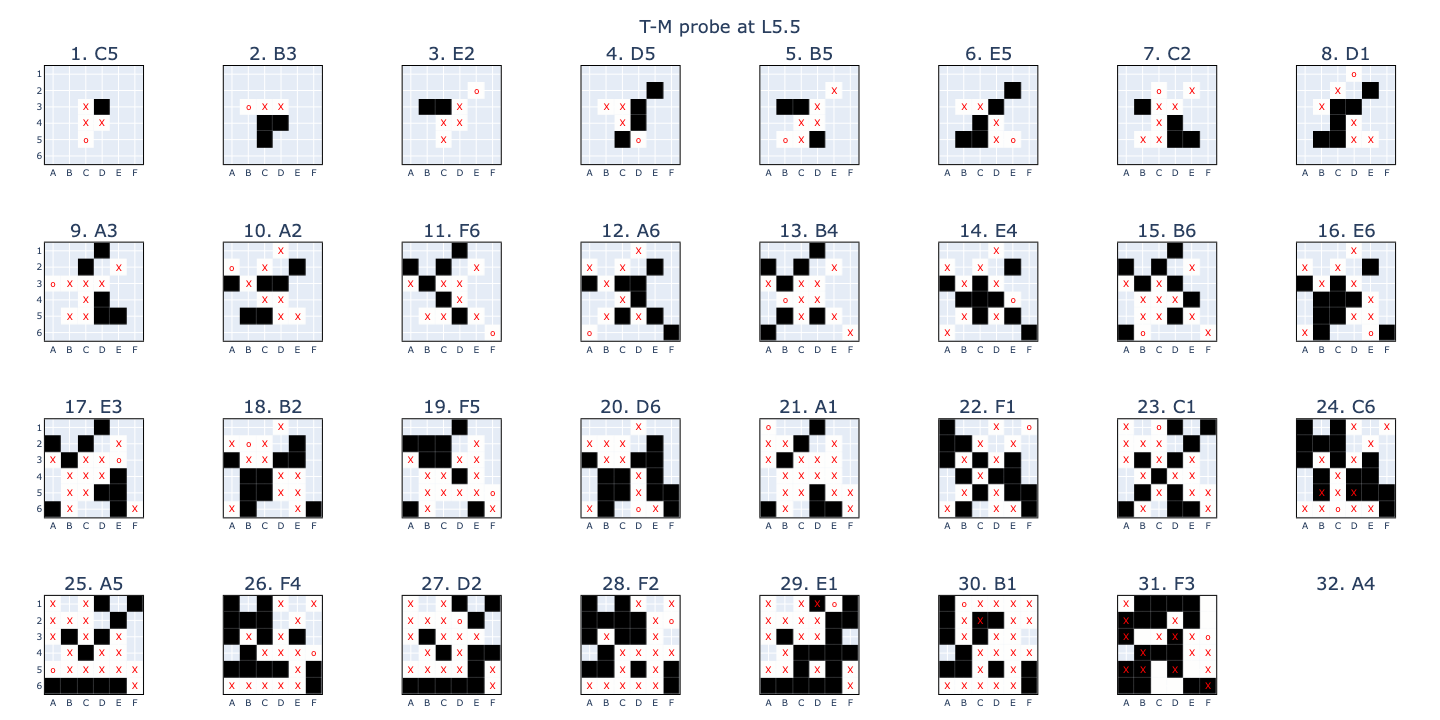
Again, success! The TEM accuracy, averaged across all inputs except the penultimate move, peaked at over 98% across L5-6. I found it informative to split each class into individual binary probes. This showed that whether a square was \(empty\) (E) could be perfectly predicted as early as L0.5! Another point of interest was that the \(theirs\) (T) accuracy was around 5% better than \(mine\) (M), equivalent to 1.8 board squares. This is probably due to the fact that the last played move in Othello, and whichever square(s) it captured, must be (T).

With these results, I decided to retrain the probes from scratch as two binary classifiers: “is this square empty?” (EE) and “is this non-empty square theirs or mine?” (TM). This was slightly different from Neel’s approach: instead of retraining, he transformed the original probes into \((E-\frac{T+M}{2})\) and \((T-M)\). I thought the high standalone accuracy of the (E) probe suggested that it could suffice as its own thing and that if we conditioned the training data for the (TM) probe such that it didn’t have to worry about empty squares, then it would be better able to isolate the salient features. The training distributions were also nice: \(P(E) = 0.5\) and \(P(T\mid\sim E) = 0.5\).

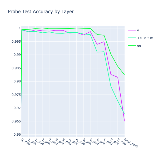
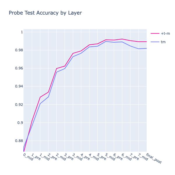
The (EE) probe outperformed the other two, but strangely the (TM) probe was less accurate than the (T-M) probe, despite being trained directly on the target data. Maybe there was some information to be gained from the empty squares, e.g. if a square’s neighbours are all empty except one, then it can’t have been flipped from its original colour. Whatever the reason, I went with the more accurate (T-M) probe going forwards.

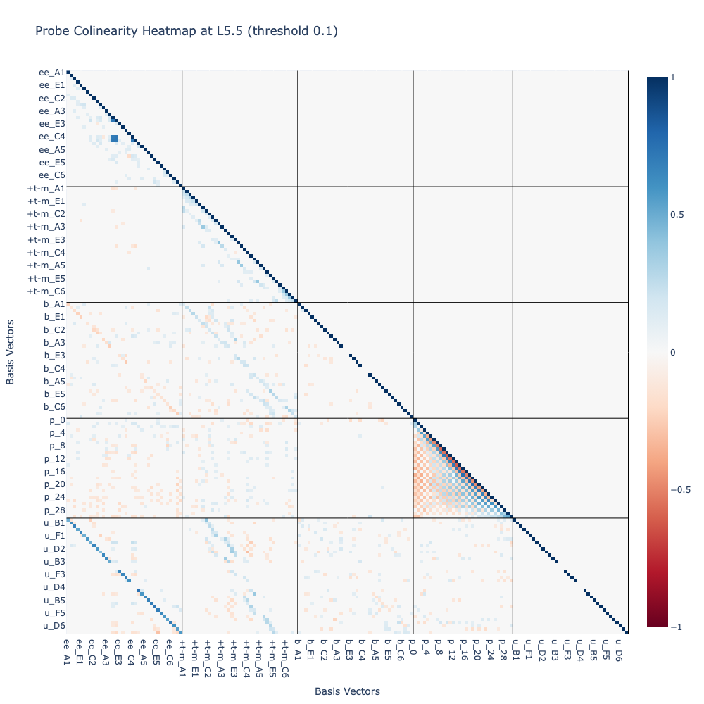
Perhaps the most informative visualisation at this stage was the colinearity (or cosine similarity) grid above. My intuition was that it would be nice to decompose the ~256 residual stream dimensions into a “canonical” basis, so I wanted to examine the orthogonality between all candidate vectors. I made the following observations:

The (EE) and (T-M) vectors were highly orthogonal, making them suitable candidates for the basis.
My intuition on weight untying seemed to be supported by high orthogonality betweeen the embedding (B) and unembedding (U) vectors.
The position embedding (P) seemed to record parity (theirs/mine) with closer positions more aligned than further ones.
It looked like there were some interesting colinearity patterns between probes of different squares in (EE).(EE), (T-M).(T-M), (B).(EE), (B).(T-M), (U).(EE), (U).(T-M).

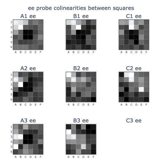
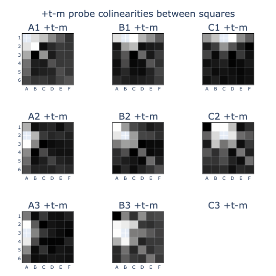
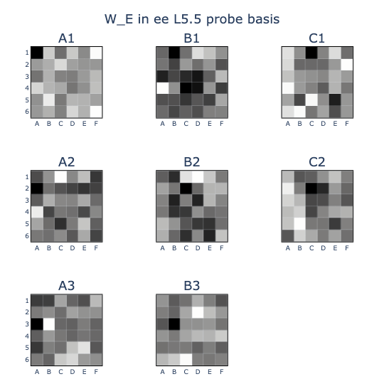
I thought that the colinearity patterns might be easier to recognise if they were rearranged into board shapes, so I did this and some cool patterns came out!

In (T-M).(T-M), the probes exhibited colinearity between squares on the same lines or diagonals, suggesting that they were frequently the same colour as one another (e.g. when just captured).
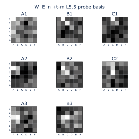
This was subtly different from the embedding weights W_E (B) in the (T-M) basis, where (B) induced a prior distribution for which squares might be captured by a move. You can see this lack of symmetry in the B2 square, which can never capture A1 but is frequently the same colour.
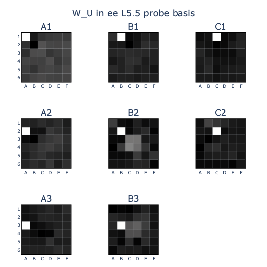
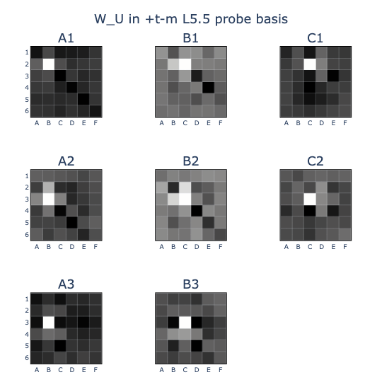
The clearest pattern was in the unembedding (U) where squares that were (EE) and had a neighbouring (T-M) backstopped by (M-T) were likely to have high logits (U). This makes sense in the causal direction, but it carries the potential issue that any circuit that writes out (U) would also write out these (EE) and (T-M) directions by correlation.

Interpreting neurons

I used these probes to replicate Neel’s discovery of modular neuron circuits. In a MLP with a single hidden layer, a neuron \(N\) can be described by the equation

\[N(\mathbf{x}) = \mathbf{w_o} \cdot GELU(\mathbf{w_i} \cdot \mathbf{x})\]

where \(\mathbf{x},\mathbf{w_o},\mathbf{w_i} \in \mathbb{R}^{d_m}\) are the residual stream vector, output weights, and input weights, respectively. If a neuron were designed to activate on the condition “A1 is empty”, it would have \(\mathbf{w_i}\) aligned with the equivalent probe vector, in this case tem_probe[..., 1, 0]. Similarly, \(\mathbf{w_o}\) could be aligned to write specific outputs to the residual stream.

We can also use the unembedding (U) and embedding (B) weights as probes, which can be interpreted as direct contributions to the output logits and direct injections of input vectors, respectively. This allows us to reverse engineer a neuron’s design by transforming its weights into probe bases.

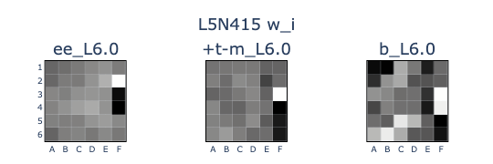
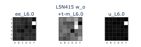
I did this to L5N415 (the 415th neuron in the 5th MLP layer), plotting the input weights (w_i) in the (EE), (T-M), and (B) bases, and the output weights (w_o) in the (EE), (T-M), and (U) bases. From the input weights, it looks like the neuron identifies boards where F2 is empty, F3 is theirs, and F4 is mine, which would make F2 legal. This is reflected in F2 being unembedded in the output weights.

But as we saw in the previous section, writing out (U_F2) also writes out (T-M_E3) and (M-T_D4), an example of the model using correlation, not causation, in its computations. This is an explanation for why the model’s board state representation degraded after L5_mid: superposition!

Conclusion

At this point, I was fairly satisfied with the replication work I’d done. I had reduced the model down to a much more manageable size, recreated the original probes, made a few slight alterations, and found a cool neuron. I think I gained three new insights from this work:

The empty probe was a perfect predictor across most of the model
Untying the embedding/unembedding weights allowed the model to align them to different, more relevant, and interpretable vectors
The degradation in board state probe performance seemed to be explained by superposition between the board state and unembedding vectors

There were a few more experiments to replicate, such as using the linear probes for causal interventions, identifying cool neurons by statistical methods, activation patching, and spectrum plots, and if you’re interested in these then you should definitely check out the ARENA tutorial.⁶

I originally intended for this to be a little side project that would allow me to practice some ML basics by replicating a paper; it was my first real foray into mech interp. However, the process of implementing my own project left me with lots of questions and I got excited about potentially answering some of them, so I decided to use Neel’s MATS application task of speedrunning a research project in 10-16 hours as a challenge for producing something new out of this project. The results of this mini-sprint will be presented in Part 2…

Feel free to fork my code⁷ if it’s at all usable, or send me an email if you have any questions or requests. I’m new to this, so I’d really appreciate any thoughts and feedback. If you got this far, thanks for reading!

References

Kenneth Li et al. (2023). “Emergent World Representations: exploring a sequence model trained on a synthetic task”. ICLR 2023. URL ↩
Kenneth Li, “Do Large Language Models learn world models or just surface statistics?”, The Gradient, 2023. URL ↩
Neel Nanda. “Actually, Othello-GPT Has A Linear Emergent World Representation”. URL ↩
Andrej Karpathy. “NanoGPT: The simplest, fastest repository for training/finetuning medium-sized GPTs.” URL ↩
Elhage, et al., “A Mathematical Framework for Transformer Circuits”, Transformer Circuits Thread, 2021. URL ↩
Neel Nanda, Callum McDougall. “ARENA [1.5.3] OthelloGPT”. URL ↩
Me. “othello-gpt” URL ↩