Hyper-Connections

Have you ever looked at a boring old RNN and thought to yourself, “I wish this looked more like a game of 5D Chess with Multiverse Time Travel”? If so, you’ll like this paper…

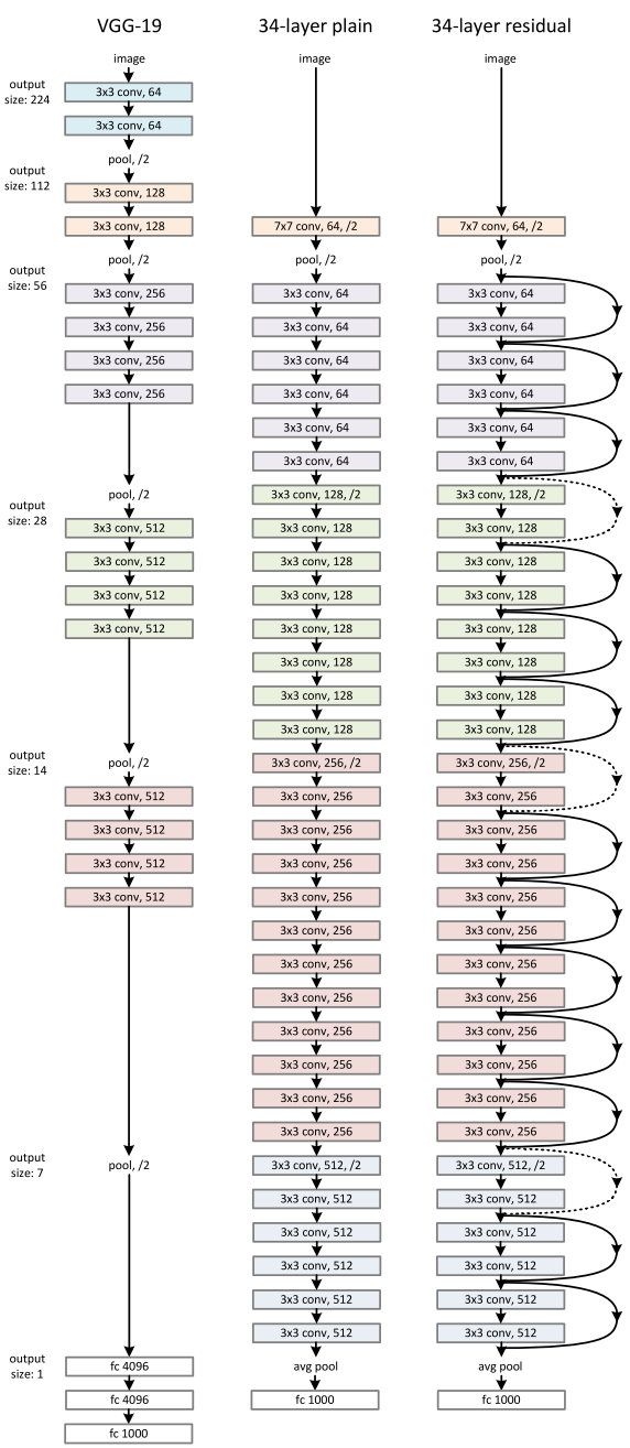
We start with a quick review of Residual Neural Networks. In a $D$-dimensional RNN with $L$ layers consisting of residual blocks $\mathcal{T}^k: \mathbb{R}^D \rightarrow \mathbb{R}^D$, each layer $k \in [1, L]$ will take an input $\mathbf{h^{k-1}} \in \mathbb{R}^D$ and compute

\[\mathbf{h^k} = \overbrace{\mathbf{h^{k-1}}}^{\text{skip}} + \underbrace{\mathcal{T}^k(\overbrace{\mathbf{h^{k-1}}}^{\text{input}})}_{\text{output}} \tag{1}\]

Hyper-Connections¹ (HC) extend RNNs by expanding the residual stream $\mathbf{h} \in \mathbb{R}^D$ into a hyper-stream $\mathbf{H} \in \mathbb{R}^{N\times D}$ with expansion factor $N$. This is done by tiling the initial input $\mathbf{h^0}$ such that $\mathbf{H^0} = \begin{pmatrix} \mathbf{h^0} & \cdots & \mathbf{h^0} \end{pmatrix}^T $. Subsequently, we introduce three linear maps for each layer that correspond to the three components of an RNN skip connection:

\[\mathbf{H^k} = \overbrace{\mathbf{A_r^k}^T\mathbf{H^{k-1}}}^{\text{hyper-skip}} + \underbrace{\mathbf{B^k}^T \mathcal{T}^k(\overbrace{\mathbf{H^{k-1}}^T \mathbf{A_m^k}}^{\text{hyper-input}})^T}_{\text{hyper-output}} \tag{2}\]

We can see that $\mathbf{A_r^k} \in \mathbb{R}^{N\times N}$ represents a hyper-skip connection, $\mathbf{A_m^k} \in \mathbb{R}^{N\times 1}$ represents a hyper-input connection, and $\mathbf{B^k} \in \mathbb{R}^{1\times N}$ represents a hyper-output connection, where each hyper-matrix forms a linear projection which connects the hyper-residual streams $\mathbf{H^k}$, $\mathbf{H^{k-1}}$ to the layers $T^k$ in a highly configurable manner.

The HC weights can be stored in a combined matrix

\[\mathcal{HC} = \begin{pmatrix} \mathbf{0_{1\times 1}} & \mathbf{B} \\ \mathbf{A_m} & \mathbf{A_r} \end{pmatrix} \in \mathbb{R}^{(n+1) \times (n+1)} \tag{3}\]

where if we set $N = 1$ and $\mathcal{HC} = \left(\begin{smallmatrix}0 & 1 \newline 1 & 1\end{smallmatrix}\right)$, we recover the original skip connection from equation (1). We can make these weights data-dependent by employing tanh-activated projections

\[\begin{align*} \mathcal{A_r}(\mathbf{H}) &= \mathbf{A_r} + s_\alpha \tanh(\mathbf{\bar{H}} \mathbf{W_r})\\ \mathcal{A_m}(\mathbf{H}) &= \mathbf{A_m} + s_\alpha \tanh(\mathbf{\bar{H}} \mathbf{W_m})\\ \mathcal{B}(\mathbf{H}) &= \mathbf{B} + s_\beta \tanh(\mathbf{\bar{H}} \mathbf{W_b})^T \end{align*}\]

where $\mathbf{W_r} \in \mathbb{R}^{D\times N}$, $\mathbf{W_m} \in \mathbb{R}^{D\times 1}$, $\mathbf{W_b} \in \mathbb{R}^{D\times 1}$ project the normalised hyper-stream $\mathbf{\bar{H}}$ into the appropriate weight spaces, and $s_\alpha$, $s_\beta$ are learned scales for the tanh-activations. The authors refer to these as Dynamic Hyper-Connections (DHC), as opposed to the original Static Hyper-Connections (SHC).

SHC allows for architectural flexibility. For example, let’s take a Transformer layer consisting of one Attention block (layer $k$) and one FFN block (layer $k+1$) with input $\mathbf{H^{k-1}} = \begin{pmatrix} \mathbf{h_1} & \mathbf{h_2} \end{pmatrix}^T$, and set

\[\begin{align*} \mathcal{HC^k} &= \begin{pmatrix} 0 & 1 & 0 \\ 1 & 1 & 1 \\ 1 & 1 & 1 \end{pmatrix}\\ \mathcal{HC^{k+1}} &= \begin{pmatrix} 0 & 0 & 1 \\ 0 & 1 & 0 \\ 1 & 0 & 1 \end{pmatrix}\\ \end{align*}\]

graph LR %% COLOR CLASSES classDef attn fill:#CCF,stroke:#000,color:#000 %% Attn module classDef ffn fill:#FFC,stroke:#000,color:#000 %% FFN module classDef h1 fill:#E8F0FF,stroke:#444,color:#000 %% Stream 1 states classDef h2 fill:#FFF4DD,stroke:#444,color:#000 %% Stream 2 states classDef zero stroke-dasharray:4 4,stroke:#666,color:#666 %% zero-weight edges classDef block fill:#FFEAB5,stroke:#000,color:#000 %% yellow block containers %% ===== INPUT STATES ===== H1["h₁"]:::h1 H2["h₂"]:::h2 %% ===== ATTENTION BLOCK (yellow container) ===== subgraph AttnBlock[" "] class AttnBlock block direction LR A_in["a_in"]:::h1 Attn["Attn"]:::attn A_in --> Attn end %% ===== Edges into ATTENTION BLOCK ===== H1 -->|1| A_in H2 -->|1| A_in %% ===== INTERMEDIATE STATES ===== H1p["h₁′"]:::h1 H2p["h₂′"]:::h2 %% Ar_odd: state→state (all 1s) H1 -->|1| H1p H1 -->|1| H2p H2 -->|1| H1p H2 -->|1| H2p %% B_odd: Attn→states Attn -->|1| H1p Attn -.->|0| H2p:::zero %% ===== FFN BLOCK (yellow container) ===== subgraph FFNBlock[" "] class FFNBlock block direction LR F_in["f_in"]:::h1 FFN["FFN"]:::ffn F_in --> FFN end %% ===== Edges into FFN BLOCK ===== H1p -.->|0| F_in:::zero H2p -->|1| F_in %% ===== OUTPUT STATES ===== O1["h₁″"]:::h1 O2["h₂″"]:::h2 %% Ar_even: state→state H1p -->|1| O1 H2p -->|1| O2 H1p -.->|0| O2:::zero H2p -.->|0| O1:::zero %% B_even FFN -.->|0| O1:::zero FFN -->|1| O2

Fig 2. Parallel configuration of SHC weights

We see that $\mathbf{a_{in}} = \mathbf{f_{in}} = \mathbf{h_1} + \mathbf{h_2}$, so the blocks are effectively applied in parallel, as if we had a Parallel Transformer architecture with a single residual stream.

Other architectural changes could include complete ablation of certain blocks or the re-injection of earlier residuals into later layers, both of which are observed in the paper.

graph LR classDef attn fill:#CCF,stroke:#000,color:#000 classDef ffn fill:#FFC,stroke:#000,color:#000 classDef h1 fill:#E8F0FF,stroke:#444,color:#000 classDef h2 fill:#FFF4DD,stroke:#444,color:#000 %% INPUT H_in["h₁, h₂"]:::h1 %% PARALLEL BLOCK subgraph Parallel_Block direction LR %% Stream 1 (Attn) subgraph S1[ ] direction TB A_in["a_in"]:::h1 Attn["Attn"]:::attn H1mid["h₁′"]:::h1 A_in --> Attn --> H1mid end %% Stream 2 (FFN) subgraph S2[ ] direction TB F_in["f_in"]:::h2 FFN["FFN"]:::ffn H2mid["h₂′"]:::h2 F_in --> FFN --> H2mid end end %% OUTPUT H_out["h₁″, h₂″"]:::h1 %% INPUT SPLIT H_in --> A_in H_in --> F_in %% OUTPUT MERGE H1mid --> H_out H2mid --> H_out

Fig 3. Parallel Transformer

DHC allows for data-specific gating. For example, maybe one hyper-stream could process grammatical features while another focused on word predictions.

Of course, the hyper-streams come with some overhead. The additional parameter count is negligible: vanilla Transformer parameter counts are $\mathcal{O}(D^2L)$, while SHC adds $\mathcal{O}(N^2L)$ and DHC adds $\mathcal{O}(DNL)$, with $N \ll D$. Similarly, the computational overhead is also small, since the weights are low-rank. The main overhead comes from the additional activations produced by the hyper-stream, amounting to a significant +16% for HCx2 and scaling approximately linearly with $N$.

In order to alleviate the memory overhead, the authors propose Frac-Connections² (FC), where instead of expansion rate $N \geq 1$, we employ a frac-rate $M = 1/N \geq 1$ that shards the input into $M$ chunks: $ \mathbf{F^0} = \begin{pmatrix} \mathbf{h^0_1} & \cdots & \mathbf{h^0_M} \end{pmatrix}^T = \text{Reshape}(\mathbf{h^0}, (F, M))$ where $F = D/M$. Instead of summing projections of hyper-streams, we now concat projections of chunks to form the inputs to the blocks, which means that $\mathbf{A_m}$ is now a square matrix, but otherwise the connection layout is similar to that of HC.

Unfortunately (and slightly suspiciously), the authors don’t offer much in terms of like-for-like comparison between the two architectures (all we have to go on is a small graph plotting DFC training loss over 3T tokens vs DHC on just 0.5T tokens), so this is something I’ll have to pursue in the replication. However, it is shown that DFC outperforms vanilla architectures with minimal overhead.

Thoughts ¶

Avoiding representation collapse is presented as the primary motiviating factor for HC. But sometimes it can be useful. E.g. OthelloGPT forgetting board state representation in final layers to replace with legality (yes, this is a toy example, but possibly similar to some language subtasks).
Authors claim that low cosine similarity between layers supports the case for HC. This is a potentially misleading proxy for usefulness - if we replaced the hyper-streams with random noise then this would also decrease similarity. Rather, it could be more informative to perform model ablations, such as dropping out entire layers.
Architectural reconfiguration is valuable, but this is essentially a hyperparameter search in a large, combinatorial space. Simple gradient descent run alongside the rest of the model training might not necessarily converge to a good solution (that being said, empirically it seems to do OK).
The case where certain connection weights tend to 0 is reminiscent of Edge Pruning in mech interp!³ However, I would intuit that circuit discovery is a much more suitable use case as the underlying subtask is simpler than that of a full LLM.
Expanding beyond $N=2$, the minimum requirement for parallel architectures, seems unnecessary. The $\mathbf{A}$ matrix “width connections” seem a little redundant as relative rescaling can be done within the Transformer blocks. I can anecdotally back this up by observing most of the performance gains in my replication when using DHC/DFC with $N=M=1$. Also, the success of frac-connections further suggests that maybe the “hyper-“ approach is unnecessary. The common denominator across hyper- and frac-connections is the dynamic element.
The authors have a small section presenting the DHCx1 model as a “failure” because it ablates an Attention block and converges slower. However, it ends up with pretty much the same performance as the control model, so I actually see this as a success!
Both hyper-/frac-connections can be thought of as full-/low-rank projections where $\mathbf{\Lambda_1} = \mathbf{\Lambda_2} = \mathbf{I}$, $\mathbf{\Gamma_1} = \begin{pmatrix} \mathbf{I_F} & \mathbf{0_F} \end{pmatrix}$, $\mathbf{\Gamma_2} = \begin{pmatrix} \mathbf{0_F} & \mathbf{I_F} \end{pmatrix}$, and

\[\begin{align*} \mathbf{H^0} &= \begin{pmatrix} \mathbf{h^0} & \mathbf{h^0} \end{pmatrix}^T = \begin{pmatrix} \mathbf{\Lambda_1} \mathbf{h^0} & \mathbf{\Lambda_2} \mathbf{h^0} \end{pmatrix}^T\\ \mathbf{F^0} &= \begin{pmatrix} \mathbf{h^0_1} & \mathbf{h^0_2} \end{pmatrix}^T = \begin{pmatrix} \mathbf{\Gamma_1} \mathbf{h^0} & \mathbf{\Gamma_2} \mathbf{h^0} \end{pmatrix}^T \end{align*}\]

Any linear operations outside of the non-linear Transformer blocks may be folded into each other. This may provide insights into generalisation and/or equivalences. What if we set $M = D$??
I replicated the paper! Repo is here. Pending $$$ to pre-train on 3T tokens…

References ¶

Zhu, D., et al. (2024). Hyper‑Connections. arXiv:2409.19606. ↩
Zhu, D., et al. (2025). Frac‑Connections: Fractional Extension of Hyper‑Connections. arXiv:2503.14125. ↩
Bhaskar, A., Wettig, A., et al. (2025). Finding Transformer Circuits with Edge Pruning arXiv:2406.16778 ↩