[Blogtober #5] Modeling survival

When will I die?
This question motivates a branch of statistics called survival analysis, aimed at predicting the time until failure for continuous processes. It has wide-reaching applications, ranging from insurance to medicine, automotive engineering, and economics.
We formulate the problem mathematically by representing the time to event as a real-valued, non-negative random variable \(T\). Given the cdf \(F(t) = \mathbb{P}(T\leq t)\), we refer to the survival function as the complement \(S(t) = 1 - F(t)\). This can either be interpreted as the likelihood that an individual survives past time \(t\), or the expected proportion of a population remaining at time \(t\).
Individualised predictions 
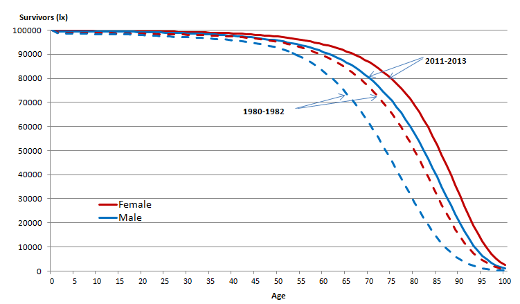
Commonly, we want to condition the survival function on some features \(X\). For example, in the graph above, the function changes based on year and gender. This is simple enough for categorical features, but suppose we want to use continuous variables such as age, weight, and height. How do we incorporate this in a sensible manner?
One way to do this is by assuming \(F\) is differentiable, such that \(f(t) = F'(t)\), and defining a hazard function \(h(t) = {f(t)}/{S(t)}\). This represents the instantaneous chance of failure at time \(t\) for any current survivors, which is a more intuitive value. For example, in radioactive decay, this would be the chance of an atom splitting at a given point in time.
The simplest hazard function is constant over time, \(h(t) = \lambda\). Since
\[\frac{d}{dt} \log S(t) = \frac{-f(t)}{S(t)} = -h(t)\]we can see that this corresponds to the Exponential distribution \(S(t) = \exp(-\lambda t)\). Now, we can condition on inputs by letting \(\lambda = \lambda(x)\).
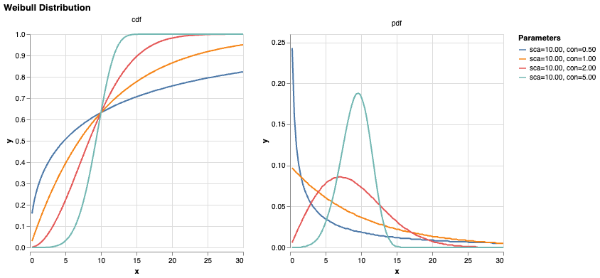
We can introduce time dependence with the cumulative hazard function \(H(t) = (t/\theta)^k\), where we refer to \(\theta\) as the ‘scale’ parameter and \(k\) as the ‘shape’ or ‘concentration’. Then
\[S(t) = \exp(-H(t))\] \[f(t) = h(t)\exp(-H(t)) = \frac{k}{\theta} \left(\frac{t}{\theta}\right)^{k-1} \exp\left[-\left(\frac{t}{\theta}\right)^k\right]\]assuming S(0) = 1. This is known as the Weibull distribution. If \(k=1\), the hazard is constant over time, i.e. the Exponential distribution; if \(k<1\), then it decreases over time, and vice versa. [TODO] medical intuition for each case.
Again, by letting the parameters \(\theta\) and \(k\) be functions of \(x\), we allow each case to have its own predicted survival curve.
Right-censored data 
In order to train these parameter mappings, we want to use maximimum likelihood estimation over a dataset \(\mathcal{D}\). However, clinical trials often don’t observe patients ad infinitum, so the actual data point we receive for a patient might just be something like ‘during the study period from 2020-2025, the subject remained healthy’. All we can say is that \(T > 5\); any events to the right of this cutoff (censoring) time are indistinguishable. This is known as right-censoring.
Incorporating this into the likelihood isn’t mathematically challenging.
\[\mathbb{P}(T=t|C=c) = \begin{cases} f(t) & \text{if } t \leq c \\ S(t) & \text{if } t > c \end{cases}\]Let’s see what this does to our parameter estimation on a population level.
Let \(\mathcal{D} = \{D, Y\}\) represent the evidence where \(d_i = \mathbb{I}[t_i < c_i]\), \(y_i = \min(t_i, c_i)\). If the data follows an Exponential distribution, then \(F(y) = 1 - \exp(-\lambda y)\), \(f(y) = \lambda\exp(-\lambda y)\), and the likelihood
\[\mathcal{L}(\lambda \mid \mathcal{D}) = \prod_i\left[d_i f(y_i) + (1-d_i) S(y_i)\right] = \lambda^{\sum_i d_i} e^{-\lambda \sum_i y_i}\]With a conjugate Gamma prior, we have
\[\pi(\lambda) \propto \lambda^{\alpha_0-1} e^{-\lambda_0\lambda}\]and so the posterior distribution \(\pi(\lambda \mid \mathcal{D}) \sim \text{Gamma}\left(\alpha_0+\sum_i d_i, \lambda_0+\sum_i y_i\right)\), and
\[\hat\lambda_{MAP} = \frac{\alpha_0 + \sum_i d_i - 1}{\lambda_0 + \sum_i y_i}\] \[\hat\lambda_{MLE} = \frac{\sum_i d_i}{\sum_i y_i}\]As we increase the proportion of right-censored data, \(\sum_i d_i \rightarrow 0\) and \(\sum_i y_i \rightarrow \sum_i c_i > \sum_i t_i\), so \(\hat\lambda\) decreases, as expected!
One interesting follow-on question is how we should treat left-censored data, i.e. cases where someone was already diagnosed with a disease before the study started. We need to be careful to avoid look-ahead bias with our features, as \(x\) may represent data taken at \(t=0\).
Rare events 
Another common property of medical data is that events are very rare among the general population. For example, while around 1 million people in the UK (population 70 million) have dementia, over a third of cases are estimated to be undiagnosed (source). This means that less than 1% of cases in census data will be labeled as events.
We could express this by letting \(\lambda(x) \gg c\) in most cases, but this is intuitively a bit strange. For example, a genetic disease may have zero chance of over occuring in a given individual. Instead, it feels much more natural to split this off into a new parameter \(\alpha \in [0, 1]\) such that \(F(t) \rightarrow \alpha\) as \(t \rightarrow \infty\). This is how we get to our final parametric model that I’m currently using to model rare neurological diseases!