[Blogtober #3] Efficient attention - Part 1: Building blocks
This series will cover some attention adaptations that may have helped to grow LLM context sizes from 1024 tokens in GPT2 to 2 million in Gemini 1.5 Pro.
Vanilla attention 
A (causal) attention head takes an input matrix \(X \in \mathbb{R}^{N \times D}\), consisting of \(N\) tokens embedded into \(D\)-dim space, and enriches each token embedding using information from previous tokens. The amount of information transferred from token \(i\) to \(j\) is given by a scalar \(A_{ij}\) within the \(N\times N\) attention matrix A. I’m sure you’re familiar with the formulation:
\[Q = X W_Q, K = X W_K, V = X W_V\] \[A = \text{softmax}\left(\frac{QK^T}{\sqrt{d_k}}\right)\] \[Z = AV, Y = Z W_O\]where \(W_Q,W_K,W_V \in \mathbb{R}^{D\times H}\) are model weights which project \(X\) into \(H\)-dim query/key/value space. The cosine similarities between each token pair’s query and key vectors are normalised to form the attention matrix \(A\), which is in turn used to calculate a weighted average of the value vectors \(Z\), which is finally projected back into \(D\)-dim space by \(W_O \in \mathbb{R}^{H\times D}\).
Let’s count the matrix multiplications.
- \(Q,K,V\): \(3NDH\)
- \(A\): \(N^2H\)
- \(Z\): \(N^2H\)
- \(Y\): \(NHD\)
We can see that the computational complexity grows as \(\mathcal{O}(N^2)\) with sequence length. Even worse, during auto-regressive generation, the sequence length grows with each iteration! Each time we generate a new token, it is appended to the sequence and the entire attention pattern is recalculated on the new sequence. Thus, generating a sequence of length \(N\) is \(\mathcal{O}(N^3)\).
KV caching 
Fortunately, during inference, there are repetitions that can be exploited to reduce the computational load. The animation below shows how an attention pattern is calculated during inference time as a 6-token sequence is generated.
We can see that with each new token, a new row gets added to the attention matrix. In order to calculate the values along this row, only the query vector for the new token is required. On the other hand, all key vectors, including the one corresponding to the new token, are needed. However, we can see that these key vectors are largely re-used from previous iterations!
If we maintain a cache of key vectors as we go, all we need to do is append the latest key and multiply by the latest query to get the new row. There’s no need to recalculate the rest of the attention matrix because they aren’t required to generate the next token in the sequence. We apply similar reasoning to the value vectors, which we multiply by the attention pattern to get the output.
How much computation did this save? We essentially removed an order of \(N\) from each step, so now sequence generation is \(O(N^2)\)! Note: most sources refer to vanilla attention as quadratic and KV-cached attention as linear; this is the inference-time complexity for each individual token generation assuming that the KV-cache has been pre-filled up to the current token.
However, there is a trade-off here: the KV cache uses memory, growing linearly with sequence length. Using float32, 32 layers and 32 heads, each with 128-dim key/value vectors (numbers taken from Mistral 7B), each token occupies around 1MB in the KV cache. Ignoring model weights and other elements, this would allow roughly 80,000 tokens to fit on an H100 with 80GB of VRAM.
Researchers have come up with several ways to get around this, all of which can be grouped into two categories:
- Reduce the number of KV vectors that need to be cached
- Reduce the size of the KV vectors that are cached
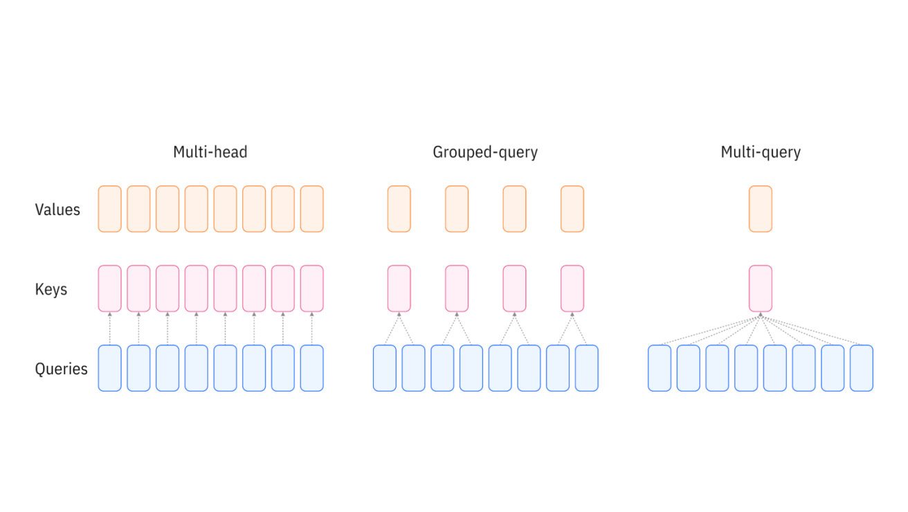
Grouped Query Attention 
Attention blocks usually consist of multiple attention heads, where each head operates as described above, but in parallel with the others. Naturally, this increases the compute and memory requirements by a multiplicative factor.
GQA is a method for reducing the number of KV vectors that need to be cached in multi-head attention by forming groups, where multiple heads query the same KV vectors. This reduces the KV cache by whatever the group size is set to, balancing expressiveness against space complexity. If the grouped heads would have had similar KV vectors anyway, the degradation in performance should be minimal.
Quantization 
Floating point values can be reduced to 16-bit precision, or even 8-bit and below. This can naively reduce the size of the KV vectors, but the impact on performance is unpredictable. A recent paper explored this idea in detail, for example by tuning each layer’s precision based on its sensitivity to changes, and purportedly managed to scale to a 10 million context length on an 8-GPU system. I’d like to do a paper review on this later.
Low-rank projection 
Linformer argues that softmax is effectively a low-rank operation, due to the fact that most values in the vector get normalised to near-0 values. This allows us to down-project each KV vector into some lower rank, reducing the size of the KV cache.
Joint compression 
Deepseek-V2 uses a form of KV compression where all KVs within a layer are represented by a single latent vector, and each head extacts unique KVs from this latent representation using learned weights.
\[C_{KV} = X W_{DKV}\] \[K^{(i)} = C_{KV} W_{UK}^{(i)}\] \[V^{(i)} = C_{KV} W_{UV}^{(i)}\]This allows each head to work with unique KVs while compressing the cache size by a factor of \(2 n_{head} d_{head} / d_{latent}\). There is an additional amount of caching required to make this compatible with RoPE, but we’ll ignore this for now.
Sliding Window Attention 
Instead of allowing each token to attend to all previous tokens within the context length, sliding window attention restricts the lookback into a constant-sized window. This reduces inference to \(\mathcal{O}(WN)\) where \(W\) is the window size and technically allows an infinite context length! However, we lose the ability to attend globally and this has some interesting effects on how models train. For example, attention sinks, a beneficial phenomenon where attention heads tend to anchor on the first token in a sequence, are removed. This has led to some interesting research into how to train such models, e.g. here and here.
RNN interpretation 
We can also reframe the attention mechanism in order to permit linear computational complexity without the need for a KV cache. Transformers are RNNs generalises the attention operation into the form
\[Z = \text{Attention}(Q_i,K,V) = \frac{\sum_{j=1}^N \text{sim}(Q_i,K_j)V_j}{\sum_{j=1}^N \text{sim}(Q_i,K_j)}\]where \(\text{sim}(q,k) = \exp\left(\frac{q^Tk}{\sqrt{D}}\right)\) in vanilla (softmax) attention. Since softmax is a non-linear operation, it is non-separable, and so the entire \(Q_i K^T\) row must be computed before softmax is applied, and only then can we multiply by \(V\).
However, if we replace \(\text{sim}(\cdot)\) with a linearly separable, non-negative kernel such that \(\text{sim}(q,k) = \phi(q)^T\phi(k)\), then we can use the associativity of matrix multiplication to get
\[Z_i = \frac{\sum_{j=1}^N \phi(Q_i)^T\phi(K_j)V_j}{\sum_{j=1}^N \phi(Q_i)^T\phi(K_j)} = \frac{\phi(Q_i)^T \sum_{j=1}^N \phi(K_j)V_j^T}{\phi(Q_i)^T \sum_{j=1}^N \phi(K_j)}\]This permits a recurrent interpretation of the transformer, where \(S_i = \sum_{j=1}^i \phi(K_j)V_j^T\), \(U_i = \sum_{j=1}^i \phi(K_j)\), and
\[Z_i = \frac{\phi(Q_i)^TS_i}{\phi(Q_i)^TU_i}\]Thus, the recurrent state \((S_i, U_i)\) requires only constant memory and can be updated at each autoregressive step in constant time, achieving true linear complexity in sequence length.
Summary 
These techniques will serve as inspirations and/or building blocks for modern advanced Transformer architectures, such as Longformer, RetNet, Mamba, YOCO, and Titans. I’ll discuss these, as well as how to evaluate relative model performance, in a later post.